Bayesian Linear Regression
March 3, 2021

Bayesian Linear Regression
March 3, 2021
1. Introduction
In linear regression models discussed so far, we seen that both OLS regression and ML regression approaches make predictions only in batch mode, which means we need to build our prediction model from scratch each time we receive new data. Bayesian regression approach – on the other hand – enables data modelling in stream mode (which means we build our model once, and update it each time we receive new data). This advantage makes Bayesian regression a more feasible approach in real life applications. In the following sections, we discuss the Bayesian specifications of linear regression in some detail.
2. The Data
Given a dataset consists of a predictor variable \(\mathbf{X}=\{x_1..x_n\}\) and a target variable \(\mathbf{Y}=\{y_1..y_n\}\), the linear relationship between them is usually defined as:
\begin{equation}
\mathbf{Y}= w_0 + w_1 \mathbf{X}
\end{equation}
Where \(w_0\) is the bias (i.e. the intercept) and \(w_1\) is the slope. We usually refer to both parameters as \(\mathbf{w}=\{w_0,w_1\}\). In Bayesian modelling, we assume an extra noise parameter \(\epsilon\) to the above equation, which represents the errors (i.e. residuals) of our model.
\begin{equation}
\mathbf{Y}= w_0 + w_1 \mathbf{X} + \epsilon
\end{equation}
The residuals are the differences between true and predicted observations:
\begin{equation}
\epsilon_i = y_i – \hat{y}_i
\end{equation}
We assume the noise parameter \(\epsilon\) is normally distributed with zero mean and constant variance \(\sigma^2\). The noise variance \(\sigma^2\) is usually replaced by its inverter \(\beta\). The parameter \(\beta\) is called the noise precision (i.e. \(\beta = \frac{1}{\sigma^2}\)):\begin{equation}
p(\epsilon)= \mathcal{N}(0,\beta^{-1})
\end{equation}
3. The Likelihood
Having the above linear equation, we can define our likelihood function. In this context, we assume our predictor \(\mathbf{X}\) to be normally distributed:
\begin{equation}
\mathcal{L}(\mathbf{Y}|\mathbf{w},\mathbf{X},\beta)=\mathcal{N}(\textbf{Y}|f(\textbf{X},\textbf{w}),\beta^{-1})= \mathcal{N}(\mathbf{w^T X},\beta^{-1})\end{equation}
In words, the likelihood distribution is a normal distribution with mean defined as the scalar product of the predictor \(\mathbf{X}\) and the coefficients vector \(\mathbf{w}=\{w_0,w_1\}\), and variance defined as the inverse of noise precision (i.e. \(\beta^{-1}\)).
4. The Prior
The role of prior distribution is to model the vector of linear coefficients \(\textbf{w}\). For the above likelihood we need to select a conjugate prior. The prior distribution is called conjugate if it belongs to the same distributions family of the posterior (e.g. both are normal distributions). In this case, we say the prior is conjugate for the likelihood. Because the Normal (Gaussian) distributions family is conjugate to itself, we select our prior to be Gaussian with zero mean and spherical covariance:
\begin{equation}
p(\mathbf{w})= \mathcal{N}(0,\alpha^{-1}\mathbf{I})
\end{equation}Note here that the prior distribution is not a univariate normal distribution but a multivariate Gaussian distribution. the multivariate Gaussian distribution is an extension to the univariate normal distribution, where the mean is expressed by a vector of values, and the covariance is expressed by a quadratic matrix. The reason behind employing multivariate Gaussian distribution in this context is that the coefficients vector \(\mathbf{w}\) has two parameters in its shortest setting \(\{w_0,w_1\}\) (i.e. in case of a single predictor). Accordingly, modelling the coefficients vector \(\mathbf{w}\) requires a multivariate distribution. In the shortest setting of \(\mathbf{w}\), the prior distribution takes the following parameters:
\begin{equation}
\mathbf{\mu}= [0,0]\quad\quad\quad\quad\mathbf{\Sigma}= \begin{pmatrix}
\alpha^{-1} & 0\\
0 & \alpha^{-1}
\end{pmatrix}
\end{equation}In this setting, the prior mean is centered on the origin in batch (offline) mode, and is updated each time the model receives new data. The covariance is spherical (or isotropic) because we assume the predictor coefficients \(\mathbf{w}\) are independent to each other. The parameter \(\alpha\) is a predefined constant in our specifications and it’s called the prior precision.
5. The Posterior
After setting both likelihood and prior distributions, we can start learning from our data and generating posteriors. The posterior has the same PDF of the prior (multivariate Gaussian), with the following definition:
\begin{equation}
p(\mathbf{w}_{new}|\mathbf{w},\mathbf{X},\mathbf{Y})= \mathcal{N}(\mathbf{\mu}_{new},\mathbf{\Sigma}_{new})
\end{equation}Here we update the prior distribution \(p(\mathbf{w})\) with new data to get the posterior distribution \(p(\mathbf{w}_{new})\). The posterior parameters are defined as follows:
\begin{equation}
\begin{split}
\mathbf{\Sigma}_{new} & = (\mathbf{\Sigma}^{-1} + \beta \mathbf{X}^\mathbf{T} \mathbf{X})^{-1}\\
& = (\alpha\mathbf{I} + \beta \mathbf{X}^\mathbf{T} \mathbf{X})^{-1}
\end{split}
\\
\mathbf{\mu}_{new}= \mathbf{\Sigma}_{new} (\mathbf{\Sigma}^{-1} \mathbf{\mu} + \beta \mathbf{X} \mathbf{Y})\end{equation}As shown above, in order to compute the posterior distribution, we need to have initial definitions of prior precision \(\alpha\), noise precision \(\beta\), plus prior mean and covariance \(\mathbf{\mu}\) and \(\mathbf{\Sigma}\).
6. The Prediction Distribution
As you might guess, the goal of calculating the posterior model parameters \(p(\mathbf{w}_{new})\) is to make predictions of new target values \(y_{new}\). Having such parameters, we are ready to make predictions. The posterior predictive distribution \(p(y_{new})\) is a univariate normal distribution defined as follows:
\begin{equation}
p(y_{new}|\mathbf{X},\mathbf{Y},\alpha,\beta)= \displaystyle\int p(y_{new}|\textbf{X},\textbf{w},\beta)\; p(w|\textbf{Y},\alpha,\beta)\; d\textbf{w}
\end{equation}The predictive distribution moments are defined as follows:
\begin{equation}
\mu_{new} = \mathbf{\mu}_{new}^\mathbf{T} \mathbf{X} = y_{new}
\\
\sigma^2_{new} = \frac{1}{\beta} + \mathbf{X}^\mathbf{T} \mathbf{\Sigma}_{new} \mathbf{X}
\end{equation}An important note to mention here is that the prediction variance consists of two terms . The first term \(\frac{1}{\beta}\) represents the level of noise in the data, while the second term represents the level of uncertainly in the model parameters \(\mathbf{w}\). Because the data and its noise are different Gaussian distributions, their variances are additive. As data size increase, the uncertainty about the model decreases. If data size goes to infinity, the second term in this equation vanishes and the Bayesian model converges to the MLE solution. This is an important fact of Bayesian inference, if data is large enough, it swallows the prior and converges to the ML estimation.
7. Design Matrix
In the above equations, I expressed the predictor variable \(\mathbf{X}\) as itself for simplicity. However, to calculate the above distributions’ parameters, we need to represent \(\mathbf{X}\) as a design matrix \(\Phi(\mathbf{X})\). If our data consists of \(n\) observations and \(m\) predictors, the design matrix is a \([n\times m+1]\) array with the first column is \([1\times n]\) vector of ones (corresponding to the bias coefficient \(w_0\)), and the rest of the array contains the predictors’ values. As an example, if we have 3 observations \(\{(x_1,y_1),(x_2,y_2),(x_3,y_3)\}\), the linear function of \(\mathbf{X}\) and \(\mathbf{Y}\) is written in matrix form as follows:
\begin{equation}
\begin{bmatrix}
y_1\\
y_2\\
y_3
\end{bmatrix} =
\begin{bmatrix}
1 & x_1\\
1 & x_2\\
1 & x_3
\end{bmatrix}
\begin{bmatrix}
w_0\\
w_1
\end{bmatrix}
\begin{bmatrix}
\epsilon_1\\
\epsilon_2\\
\epsilon_3
\end{bmatrix}
\end{equation}Or in a compact form as:
\begin{equation}
\mathbf{Y}= \Phi(\mathbf{X})\cdot \mathbf{w}\cdot \epsilon
\end{equation}
8. The Procedure
The procedure of building an streaming Bayesian linear regression model is as follows:
- INPUTS
- predictor variable \(\mathbf{X}\)
- target variable \(\mathbf{Y}\)
- initial guesses of linear coefficients \(\{w_0,w_1\}\)
- initial guesses of prior precision and noise precision \(\{\alpha,\beta\}\)
- SETUP (Offline)
- select probabilistic distribution for the data \(p(\mathbf{Y}|\mathbf{w},\mathbf{X},\beta)\)(i.e. the likelihood)
- choose a prior distribution \(p(\mathbf{w})\) that is conjugate to the likelihood distribution
- UPDATE (Online)
- calculate the posterior distribution \(p(\mathbf{w}_{new})\) by updating the prior \(p(\mathbf{w})\)
- calculate predictive distribution \(p(y_{new})\)
- set new posterior to last prior in the next iteration
9. Evaluation (Synthetic Data)
First I ran the above algorithm on synthetic dataset. The dataset has two variables (a predictor \(\textbf{X}\) and a target \(\textbf{Y}\)). The target variable \(\mathbf{X}\) ranges in \([-1, 1]\). The linear coefficients \(\mathbf{w}= \{-0.3,0.5\}\), and the predictor noise is normally distributed around 0 with variance of \(0.04\). Hence, the target variable \(\mathbf{Y}\) is defined as:
\begin{equation}
\mathbf{Y}= -0.3 + 0.5 \mathbf{X} + \mathcal{N}(0.0,0.04)
\end{equation} By executing the above procedure to our synthetic data with one observation, we got the following probability distributions:
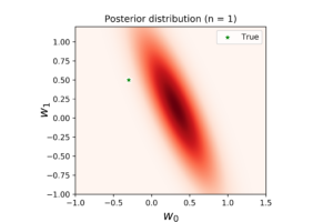
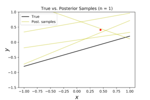
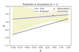
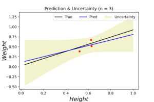
In the left figure, we note that the posterior distribution has large variance, and consequently its center is far from the true coefficients. The middle figure shows the corresponded true regression line (in black) with four randomly generated samples of the posterior (in yellow). This figure shows the high dispersity between the true and the predicted regression models. In the right figure, the predicted regression model (in blue) is far from the true model (in black). In addition, the level of uncertainty surrounding the predictive model is very high. If we increase the number of observations to 3, we get the following distributions.
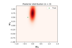
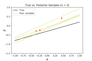
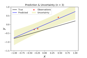
As you can see here, the posterior distribution become more dense, and the true regression model become closer to the posterior mean. The corresponded posterior samples are now less disperse and closer to the true model. This fact is translated into more accurate prediction model in the right plot.
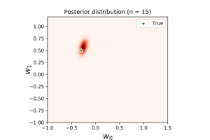
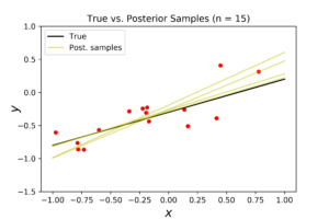
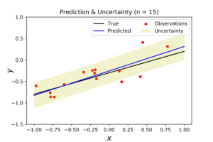
With \(n=15\) points (see above plots), the model become very close to the true regression line. This can be seen clearly from the density level of posterior distribution, the convergence of posterior samples, and the consistency of noise surrounding the predicted model.
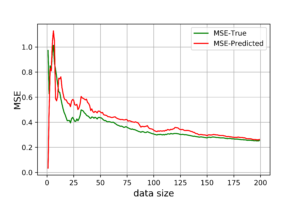
In addition, we can monitor the convergence between predicted and true regressions by measuring the mean squared error (MSE) values of both regressions. As the below figure shows, the predicted (Bayesian) regression is very noisy with small data sizes, compared to the true (OLS) regression. The larger data size, the less noisy our Bayesian regression is, until it get so close to the OLS regression accuracy (at \(n=150\)).
Prediction Interval
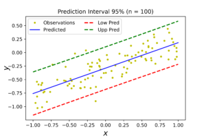
A nice tool to evaluate Bayesian regression and quantify its level of uncertainty is to draw it’s prediction interval (PI). Prediction interval quantifies the uncertainty of a given prediction model. For example, the below figure shows the prediction interval of 95% confidence of our synthetic data. It says that 95% of our model predictions are inside the range between the 2 dashed lines. As we calculate only 95% interval, some observations may lie outside that interval (i.e. outside the dashed lines).
Prediction Quality
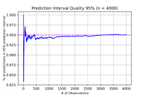
Another useful perspective to measure the correctness of our model and its embedded selections is to measure the ratio of correct predictions our model achieves over time. In the below figure, we can see that our model predictions are very close to the actual values. The model average performance has around 95% confidence level, which implies our assumptions about data distribution was correct.
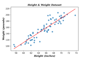
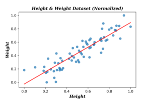
10. Evaluation (Real Data)
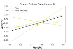
Applying Bayesian linear regression on real data is a challenging task, as we don’t know the distribution of both data and the noise surrounding it. I selected for this task a dataset of lengths and weights of random people. The following plots shows the data before and after normalization.
As for model specifications I assumed the data is normally distributed with prior precision \(\alpha= 0.5\) and noise precision \(\beta=35\). The initial guess of linear coefficients vector \(\textbf{w}=\{0.13,0.75\}\) (note: these are not the true OLE coefficients, and have been used to see how long does the algorithm take to converge). The following plots show the evaluation results at the first observation.
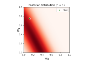
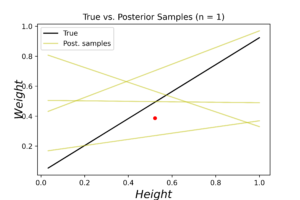
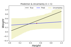
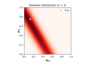
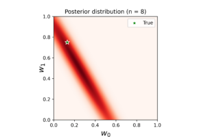
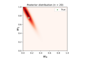
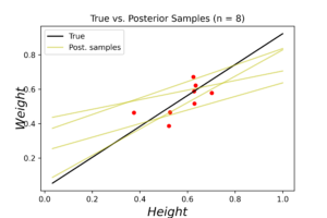
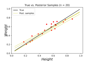
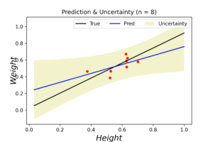
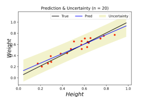
The left plot shows the posterior distribution at \(n=1\), which implies very large variance surrounding the assumed model coefficients. The middle plot shows how this variance affects the random-generated posterior samples (in yellow) when compared to the true line (in black). In the right plot we see the predicted line is way different from the true one, and comes with large level of uncertainty. By increasing the data (3, 8 and 20 points), we notice gradient convergence of the resulted posterior and predicted distributions to the true line (see the following plots). Because we don’t use the true coefficients as initial gussies, the algorithm takes longer to converge, but after 20 data points the algorithm starts to simulate the true fitted line with small level of noise.
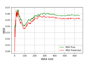
The corresponded MSE values of both true and predicted regressions are plotted below. The error range (y-axis) is small due to data normalization. Nevertheless, the noise levels are almost identical in the first few data points for both regressions. After certain threshold (\(\approx 30\) points), the noise level of true (OLE) regression starts to stabilized above the Bayesian regression for the rest of the dataset. This is an indication that the true data noise may not be normally distributed as we assumed in our model specifications.
11. Drawbacks
Although Bayesian linear regression (BLR) is a powerful tool to analyse regression problems, it has some shortcomings. Primarily, the outcome of BLR is highly dependent on our assumptions about data. This means if we make wrong assumptions about data distribution, the generated regression model will go wrong. Another shortcoming of this model is that it assumes constant noise over global data range, which may not reflect the actual noise levels for large datasets, where each region has different level of noise. A third disadvantage of this method appears when data is not normally distributed. In this case, a sophisticated Bayesian analysis need to be done to discover the data and the prior distributions with their proper initial settings.