
1. Data Aggregation
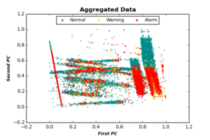
In this step, we aggregate data of all devices into one data set. Based on the output of PCA, we consider only the first 6 PCs of each event, as the remaining PCs do not add any extra information to the classification process. The selected PC features are normalized in [0,1] for each device, and aggregated into one dataset. In addition, we apply a simple moving average procedure to each class (Normal, Warning, Alarm) separately, in order to smooth classes generated after aggregation. The following figure plots aggregated data after applying simple moving average, projected by the first two PCs.
2. Imbalanced Classes
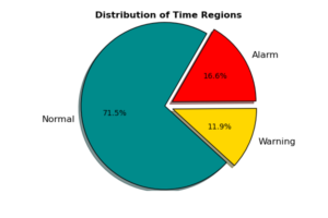
Imbalanced data classes is a common issue in many data science business domains, and predictive maintenance is not an exception. In our case, the major category of observations represents “Normal” events, where devices are running properly. This class is usually referred to as the negative class. The classes of interest however, are those classes that preceding failures (i.e. the positive classes). The following chart displays the distribution of our three classes over all devices, shows that both “Warning” and “Alarm” classes representing nearly 28% of data.
In this study, we will not balance our data by up-sampling minority classes or down-sampling the major class. This is because our ML models managed to learn minority classes properly (see below). However, if it is hard for classifiers to learn from imbalanced classes, it is recommended to balance data before training classifiers. A popular technique to treat imbalanced data classes is the up-sampling SMOTE [1] algorithm.


4. Binary Classes Evaluation
Beside validating our four classifiers in multi classification settings, we want to evaluate them as binary classifiers. The aim is to measure how each multi-class classifier performs, when it runs as binary classifier. In this section, we will not re-train each classifier with binary labeled data. Instead, we will convert the above confusion matrices into 2-d matrices, by considering both “Normal” and “Warning” classes as one majority (negative) class, and “Alarm” class as single minority (positive) class. Afterwards we evaluate all classifiers as binary classifiers.
4.1 ROC Curve
A nice visualization tool to evaluate binary classifiers is to plot the relation between the true positive (TP) and the false positive (FP) rates. The former rate specify how many “Alarm” events have been predicted correctly as “Alarms“, while the latter rate determines how many “Normal” and “Warning” events have been mistakenly predicted as “Alarms“. The significance of ROC curves is that they indicate the ability of each classifier to predict the minority class correctly (referred to as classifier sensitivity), and how much does this sensitivity influences the ability to predict majority class correctly (referred to as classifier specificity).
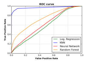
We can measure the sensitivity/specificity of each classifier by measuring the Area Under ROC Curves (AUC). As seen in the above plot, KNN classifier has the largest AUC score (0.97). This means that KNN classifier can achieve extreme high sensitivity, while keeping accurate specificity rates. The AUC value for RF classifier is (0.73), for NN is (0.62), and for Log. Regression is (0.58).
4.2 Recall-Precision Curve
Another interesting evaluation plot is the one that describes Recall and Precision trade-off for difference threshold values of each classifier. Classifier threshold is the value at which each classifier decides the label (i.e. the class) of each observation, based on the probabilistic weight it receives from each class. The following plot shows the Recall-Precision curves of the four classifiers.
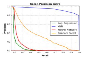
As the plot shows, all classifiers achieve high precision rates when recall is low. As recall increases, precision rates deteriorate for RF, NN, and Log. Regression classifiers. KNN classifier can — however — achieves high precision rates (around 0.9) with very high recall values (about 0.8), which makes KNN beats other classifiers in this validation criteria as well.
4.3 Calibration Curve
Calibration plot is another useful visualization tool to measure the frequency expectation of classifiers’ scores. Calibration curve of a given classifier reflects the correlation between the proportion of positive class observations scored as positive ones, and the predicted probability of positive class. Good calibrated classifiers should have high correlation between the two scales. In case of perfect calibrated classifier (one that follows the diagonal line in the below graph), if the classifier decides that a given set of observations are positive (i.e. “Alarm” events) with average probability of 0.75, then if we collect all observations with probability equals 0.75, 75% of this portion should have a true label “Alarm“. The following graph plots calibration curves of the four classifiers.
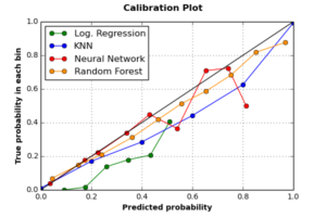
The graph shows that RF is the best calibrated classifier, followed by KNN. Although all classifiers have underestimated the true probability of observations, both RF and KNN classifiers have acceptable probabilistic estimates of the positive class. The worst calibrated classifier is Logistic Regression, as it entirely failed to estimate any positive observation correctly, followed by NN classifier, which have perfectly estimated probabilities of negative class, but ran wrongly with positive class.
4.4 Expected Cost
The last evaluation criteria in this study is called the expected cost [2]. Expected cost (or expected benefit) is a popular metric of evaluating binary classifiers. Its significance is that it binds classifier’s success and failure predictions with the corresponded benefits and costs of each prediction. Based on user’s business objectives, experts of each business domain can estimate the influence of each prediction (true negative (TN), false negative (FN), false positive (FP), and true positive (TP)). Typically, the business consequences build upon correct predictions are called benefits, while those of wrong predictions are called costs. In this study, the manufacturer assigns 0.5 benefit of true negatives, 0.99 benefit of true positives, 0.4 cost of false positives, and 0.99 cost of false negatives. The formula used for expected cost is as follows:
\begin{equation}
\begin{split}
Expected\ Cost = P(\mathbf{p})\times [P(TP)\times \textit{benefit}(TP) + P(FN)\times \textit{cost}(FN)] \\
+\ P(\mathbf{n})\times [P(TN)\times \textit{benefit}(TN) + P(FN)\times \textit{cost}(FP)]
\end{split}
\end{equation}
The values \(P(\mathbf{p})\) and \(P(\mathbf{n})\) represent probabilities of positive and negative classes respectively, and values \(P(TP), P(FN), P(TN)\) and \(P(FN)\) represent probabilities of the classifiers’ four types of predictions. By calculating the expected cost of the above four classifiers, KNN scores the lowest cost with 0.61, followed by Log. Regression (0.69), RF (0.81), and NN (0.99).
This means that from manufacturer’s business perspective, using KNN classifier shall best minimize the operational costs of his medical equipments. Based on this fact, and all other evaluation metrics above, we recommend KNN classifier as the most suited classifier for this case study.