Common Continuous Probability Distributions
Part 1
February 24, 2021

Common Continuous Probability Distributions
Part 1
February 24, 2021
1. Uniform distribution
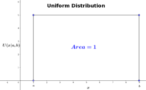
In continuous uniform distribution, the Probability Density Function (PDF) for a random variable \(x\) is constant over all values of \(x\). Like any other continuous probability distribution, the area under the graph must equal to 1. The density function of uniform distribution looks like this:
And the PDF is defined as:
\begin{equation}
U(x|a,b) =
\begin{cases}
\frac{1}{b-a}, & a\leq x\leq b \\
0, & otherwise
\end{cases}
\end{equation}
The uniform distribution of a given variable \(x\) is controlled by two parameters (\(a,b\)), representing the minimum and maximum values that \(x\) can takes respectively, where \(b>a\). No matter which value \(x\) takes, the uniform probability \(U(x|a,b)\) is constant for any \(x\in[a,b]\).
Example
As an example, suppose that for a job you applied for, you passed the first interview successfully, and the interviewer told you that the second interview will be within 2 weeks. What is the probability that the second interview will be between 10 and 12 days?
Here, we have \(a\) and \(b\) values are \(0\) and \(14\) days, such that \(x\in[0,14]\). Accordingly, we compute our PDF as follows:
\begin{align*}
U(x|a,b) = \frac{1}{b-a} = \frac{1}{14}
\end{align*}
The interval of \(x\) where the second interview lies between 10 and 12 days is \(x\in[10,12]\), with a range of \(2\) days. This means (\(b-a=2\)). The corresponded uniform probability is simply the sub-area in a rectangle where \(x\) lies between 10 and 12, multiplied by the height of that rectangle, which is \(U(x|a,b)\):
\begin{align*}
P(10\leq x\leq 12) = (12-10)\times \frac{1}{14} = \frac{1}{7} = 0.14
\end{align*}
Moments
In uniform distribution, the expectation and the variance of variable \(x\) are computed as follows:
\begin{equation}
E(x) = \mu(x) = \frac{a+b}{2};\;\;\;\;\;\;
V(x) = \sigma^2(x) = \frac{(b-a)^2}{12}
\end{equation}
because the distribution is symmetric around its mean value, the mean is equal to the median.
2. Beta distribution
Beta distribution is a probability distribution over continuous probabilistic variable \(x \in[0,1]\). In other words, it samples a distribution of probabilities (i.e. it represents all possible values of a probability). Beta distribution is controlled by two variables \(a\) and \(b\) such that both \(a>0\) and \(b>0\). The PDF of Beta distribution is defined as follows:
\begin{equation}
Beta(x|a,b) = \frac{x^{a-1}(1-x)^{b-1}}{B(a,b)}
\end{equation}
where:
\begin{align*}
B(a,b) = \frac{\Gamma(a)\Gamma(b)}{\Gamma(a+b)}\ \ ; \Gamma(a)= (a-1)!
\end{align*}
The denominator of Beta function \(B(a,b)\) is just a normalization constant to insure that the integral of \(Beta(x|a,b)\) sums up to 1. This constant is independent of \(x\).
The significance of Beta distribution is that it gives a probability estimate of \(x\) in range \([0,1]\), which makes it (from probabilistic point of view) a very suitable function to describe prior hypotheses of a given experiment before any measurements are taken. In addition, changing the values of parameters \(a\) and \(b\) gives us a wide range of shapes that identify the way we believe \(x\) is distributed.
Example
Suppose a doctor wanted to test a new flu drug on his patients. Before the new drug is tested, there is no idea of the drug success/failure rate. Therefore, we can represent the prior probability of the drug success by a Beta distribution where parameters \(a\) and \(b\) are equal to 20.
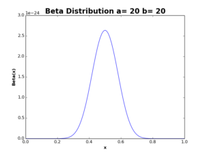
The above plot represents the prior distribution of drug success before testing the drug. As the plot shows, the expected value of \(x\) is \(0.5\), which reflects equal chance of drug’s success/failure.
Next, assume the doctor started to use the drug in his prescriptions to flu patients. After 3 months, the doctor found that out of \(100\) patients whom used the drug, \(70\) of them were recovered from flu within a week, while the rest have not been affected by the drug. Now, if we want to update our prior probability using this new data, we would update our Beta distribution to be:
\begin{align*}
Beta(x|a,b) = Beta(x|a+success,b+failure) = Beta(x|90,50)
\end{align*}
The resulting distribution is shown in the following plot:
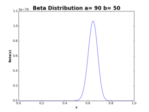
After updating Beta distribution with new data, the curve is now more thinner and shifted to the right, with increase in the mean value from \(0.5\) to \(0.64\). If we received the data of the next \(100\) flu patients, saying that \(83\) of them have been recovered after using the drug, we can update our distribution again:
\begin{align*}
Beta(x|a,b) = Beta(x|173,67)
\end{align*}
The resulting function is shown in the following plot:
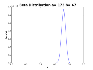
As you see, the curve is again more thinner and more shifted to the right, recording a new expected success ratio \(\mu(x)= 0.72\). The more data we use in the model, the more thinner distribution we get, and – of course – a more reliable estimation we obtain.
Moments
In Beta distribution, the expectation and the variance of probabilistic variable \(x\) are calculated as follows:
\begin{equation}
E(x) = \mu(x) = \frac{a}{a+b} ;\;\;\;\;\;\;
V(x) = \sigma^2(x) = \frac{ab}{(a+b)^2(a+b+1)}
\end{equation}
3. Dirichlet distribution
Dirichlet distribution is a probability distribution that samples a probability complex rather than a continuous variable. A probability complex is a set of probabilities that sums up to \(1\). Examples of probability complexes are: \(\{0.1,0.5,0.4\}\), \(\{0.1,0.9\}\), \(\{0.2,0.3,0.3, 0.2\}\). You can think of Dirichlet distribution as a generalization of Beta distribution, where we have a multidimensional (i.e. \(k>2\)) probabilistic space.
Having a probability complex \(\mathbf{P}= \{p_1,p_2,…,p_k\}\), the Dirichlet distribution PDF is defined as:
\begin{equation}
Dir(\mathbf{P}|\mathbf{\alpha}) = \frac{\prod_{i=1}^k p_i^{\alpha_i-1}}{B(\mathbf{\alpha})};
\quad \quad \quad \sum_{i=1}^k p_i= 1\ \&\ p_i\geq 0\ \forall\ p_i \in \mathbf{P}
\end{equation}
where \(B(\mathbf{\alpha})\) is the Beta function, and it is defined as:
\begin{align*}
B(\mathbf{\alpha}) = \frac{\prod_{i=1}^k \Gamma(\alpha_i)}{\Gamma(\sum_{i=1}^k \alpha_i)};
\quad \quad \quad \alpha_i > 0\ \forall\ \alpha_i \in \mathbf{\alpha}
\end{align*}
Selecting \(\mathbf{\alpha}\)
Dirichlet distribution is controlled by a single vector parameter \(\mathbf{\alpha}= \{\alpha_1,\alpha_2,…,\alpha_k\}\), which represents the weights corresponded to the probabilistic values of \(\mathbf{P}\). Parameter \(\mathbf{\alpha}\) is called concentration hyperparameter because is determines the distribution of values generated by Dirichlet distribution. If \(\mathbf{\alpha}\) is small (i.e. \(\mathbf{\alpha}<1\)), the resulting distribution is sparsely distributed, with most values having a probability close to zero. If \(\mathbf{\alpha}\) is large (i.e. \(\mathbf{\alpha}>1\)), the resulting distribution will be more concentrated toward the center of the simplex. If \(\mathbf{\alpha}=1\), the resulting values will be evenly distributed.
Example
Suppose I give you a box contains apples of three colors: yellow, green, and red, and ask you to select random apple without looking at the box. In this case, we have three possible outcomes \(\mathbf{P}=\{p_{yellow},p_{green},p_{red}\}\).

If the amount of apples of each color is equal, then the probability of picking an apple of any color is also equal (i.e. \(p_{yellow}=p_{green}= p_{red}= \frac{1}{3}\)). However, if half of apples in the box are red, then the probability distribution would change (\(p_{red}= \frac{1}{2},\ p_{yellow}=p_{green}= \frac{1}{4}\)).
Regardless of the amount of apples of each color, we need to know the probabilistic density of every possible value of each \(p_i\in\mathbf{P}\). In order to achieve this goal, we consider each probability \(p_i\) as an independent variable. Accordingly, \(\mathbf{P}\) is a vector in \(3\) dimensional space. As the multinomial distribution requires that these three probabilities sums up to \(1\), the allowable values of \(\mathbf{P}\) end up to \(3d\) triangle:
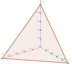
The Dirichlet distribution help us to learn the probability density at any point of this triangle, by controlling the weight parameter \(\alpha_i\) corresponded to each probability \(p_i\).
Case 1: \(\mathbf{\alpha} < 1\)
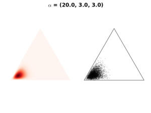
If we select hyperparameter \(\mathbf{\alpha}<1\), the resulting Dirichlet distribution will be concentrated on extreme probability values of \(\mathbf{P}\), resulting a triangle of the following shapes.
In the above figures, the color scale moves from white (lowest values) to red (highest values). This means the distribution concentrates in the corners and along the boundaries of the simplex. We select this\(\mathbf{\alpha}\) setting when we have a strong prior believe that the probability of single event dominates probabilities of all other events. As in our example, we use it if we believe that most apples in the box are of one color.
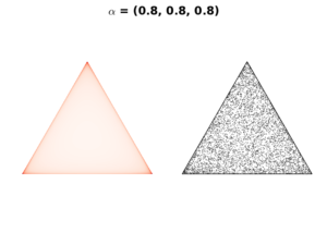
Case 2: \(\mathbf{\alpha} > 1\)
In case \(\mathbf{\alpha}>1\), the resulting distribution is concentrated to the simplex center. As \(\mathbf{\alpha}\) value increases, the distribution is more tightly concentrated on the center, as in the following figures:
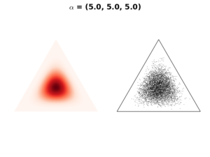

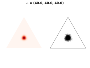
We use this setting when we have a prior believe that any event is equally likely to occur. In our example, each apple color has the same chance to be selected.
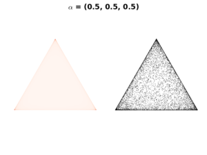
Case 3: \(\mathbf{\alpha} = 1\)
In this case, the resulting distribution will be a uniform one, where all probabilities of all events are equally likely to occur.
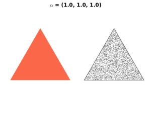
We choose \(\mathbf{\alpha}=1\) when we have no prior believe about the expected outcome.
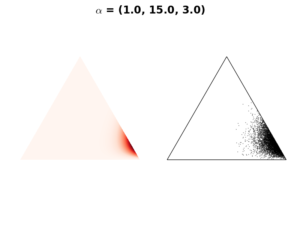
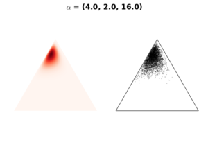
Case 4: Biased \(\mathbf{\alpha}\)
If we have a prior believe that the probability of one event to occur is much higher than all other probabilities, we can increase the chance of this event by increasing the weight of \(\alpha_i\) corresponded to this particular event. This option generates a distribution that is more concentrated on one event than the others (see the following figures).
Moments
In Dirichlet distribution, the expectation, variance and co-variance are computed as follows:
\begin{align*}
E(p_i) = \mu(p_i) = \frac{\alpha_i}{\alpha_0} ;\ \ \ \alpha_0= \sum_{j=1}^k \alpha_j
\end{align*}
\begin{align*}
V(p_i) = \sigma^2(p_i) = \frac{\alpha_i(\alpha_0 – \alpha_i)}{\alpha_0^2(\alpha_0+1)}
\end{align*}
\begin{align*}
COV(p_i,p_j) = \frac{-\alpha_i\alpha_j}{\alpha_0^2(\alpha_0+1)}\ \forall i\neq j
\end{align*}