Bayesian Data Modelling
(MLE & MAP)
February 3, 2021
Bayesian Data Modelling
(MLE & MAP)
February 3, 2021
1. Data Modelling
Data modelling is a very common terminology in software engineering and other IT disciplines. It has many interpretations and definitions depending on the field in discussion. In data science, data modelling is the process of finding the function by which data was generated. In this context, data modelling is the goal of any data analysis task. For instance if you have a \(2d\) dataset (see the figures below), and you find the 2 variables are linearly correlated, you may decide to model it using linear regression.
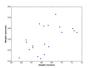
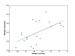
Or if you visualize your data and find out it’s non-lineary correlated (as the following figures), you may model it using nonlinear regression.
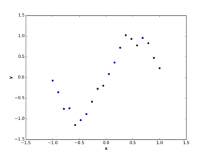
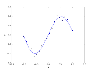
The way you find those functions is what machine learning is all about! Now, as you know what data modelling is, let’s see how we model data using the Bayesian settings.
2. Bayesian Data Modelling
Bayesian data modelling is to model your data using Bayes Theorem. Let us re-visit Bayes Rule again:
\begin{equation}
P(H|E) = \frac{P(E|H) \times P(H)}{P(E)}
\end{equation}
In the above equation, \(H\) is the hypothesis and \(E\) is the evidence. In the real world however, we understand Bayesian components differently! The evidence is usually expressed by data, and the hypothesis reflects the expert’s prior estimation of the posterior. Therefore, we can re-write the Bayes Rule to be:
\begin{equation}
P(posterior) = \frac{P(data|\theta) \times P(prior)}{P(data)}
\end{equation}
In the above definition we learned about prior, posterior, and data, bout what about \(\theta\) parameter? \(\theta\) is the set of coefficients that best define the data. You may think of \(\theta\) as the set of slope and intercept of your linear regression equation, or the vector of coefficients \(w\) in your polynomial regression function. As you see in the above equation, \(\theta\) is the single missing parameter, and the goal of Bayesian modelling is to find it.
3. Bayesian Modelling & Probability Distributions
Bayes Rule is a probabilistic equation, where each term in it is expressed as a probability. Therefore, modelling the prior and the likelihood must be achieved using probabilistic functions. In this context arise probability distributions as a concrete tool in Bayesian modelling, as they provide a great variety of probabilistic functions that suits numerous styles of discrete and continuous variables. An introductory article about probability distributions and their features can be found here.
In order to select the suitable distribution for your data, you should learn about the data domain and gather information from previous studies in it. You may also ask an expert to learn how data is developed over time. If you have big portions of data, you may visualize it and try to detect certain pattern(s) of its evolving over time, and select your probability distribution upon.
4. Maximum Likelihood Estimation (MLE)
Maximum Likelihood Estimation (MLE) is the simplest way of Bayesian data modelling, in which we ignore both prior and marginal probabilities (i.e. consider both quantities equal to 1). The formula of MLE is:
\begin{equation}
P(posterior) \propto P(data|\theta)
\end{equation}
The steps of MLE are as follows:
- Select a probability distribution that best describes your data
- Estimate random value(s) of \(\theta\)
- Tune \(\theta\) value(s) and measure the corresponding likelihood
- Select \(\theta\) that correspond to the maximum likelihood
Example
“a company captures the blood glucose (BG) levels of diabetics, analyse these levels, and send its clients suitable diet preferences. After one week of inserting her BG levels, a client asked the company smart app whether she can consume desserts after her lunch or not? By checking her after-meal BG levels, it were {172,171,166,175,170,165,160}. Knowing that the client after-meal BG should not exceed 200 mg/dl, what should the app recommend to the client?“
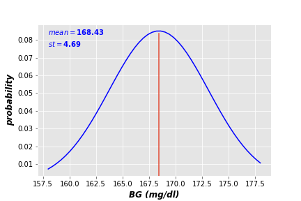
The goal here is to estimate an average BG level for the client to use it in the company recommendation system. Having the above BG sample data, we assume these readings are drew from a normal distribution, with a mean of 168.43 and standard deviation of 4.69 (see the following figure)
Now we calculate the likelihood of this estimation as follows:
\begin{equation}
\begin{split}
P(data|\theta) & = P(\{172,171,166,175,170,165,160\}|168.43)\\
& = P(172|168.43)\times P(171|168.43)\times P(166|168.43)\times P(175|168.43)\\
& \times P(170|168.43)\times P(165|168.43)\times P(160|168.43)
\end{split}
\end{equation}
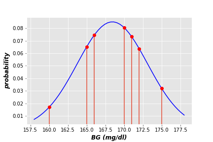
As you can imagine, multiplying small probability values (red dots in the above figure) generates very small value (very close to 0). Therefore, we replace multiplication with summation. In the above case, the sum of these probabilities equal 0.406:
\begin{equation}
\begin{split}
P(data|\theta) & = P(\{172,171,166,175,170,165,160\}|168.43)\\
& = P(172|168.43)+ P(171|168.43)+ P(166|168.43)+ P(175|168.43)\\
& + P(170|168.43)+ P(165|168.43)+ P(160|168.43) = 0.406
\end{split}
\end{equation}
In order to find the maximum likelihood, we need to estimate different values of BG levels and calculate the corresponding likelihoods. The BG value with maximum likelihood is the most suitable estimation of the BG.
To automate this process, we generate 1000 random numbers in the same range of captured BG levels, and measure the corresponded likelihoods. The results are illustrated in the following plot.
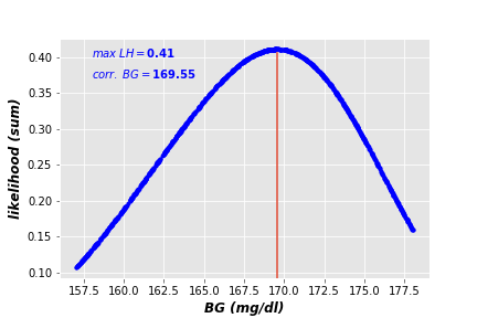
As you can see, the maximum likelihood estimate of randomly generated BGs equals 169.55, which is very close to the average of captured BG levels (168.43). The difference between both values is due to the small size of captured data. The larger sample size you have, the smaller difference between both estimates you get.
Based on this estimate, the app can recommend it’s patient to consume a small piece of dessert after at least 3 hours of her lunch, with taking the suitable insulin dose.
5. Maximum A Posteriori (MAP)
Maximum A Posteriori (MAP) is the second approach of Bayesian modelling, where the posterior is calculated using both likelihood and prior probabilities.
\begin{equation}
P(posterior) \propto P(data|\theta)\times P(Prior)
\end{equation}
You can think of MAP modelling as a generalization of MLE, where the likelihood is approximated with prior information. Technically speaking, we deal with our data samples as if it were generated by the prior distribution:
\begin{equation}
P(posterior) \propto P(data|\theta)\times P(\theta)
\end{equation}
Example
” … suppose that the client updated the app with her historical BG levels for the last month, which turned out to be 171 mg/dl on average, with standard deviation of 3, how the app can use this new information to update the patient’s BG level? “
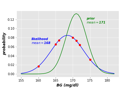
In this case, we have two distributions of Blood Glucose, one of recent data (the likelihood), and the other of historical data (the prior). Each data source can be expressed as normal distribution (see the following figure).
The posterior here is updated by multiplying the prior marginal probability by each term of data probabilities:
\begin{equation}
\begin{split}
P(data|\theta) & = P(\{172,171,166,175,170,165,160\}|\theta)\times P(\theta)\\
& = P(172|\theta)\times P(\theta)\times P(171|\theta)\times P(\theta)\times P(166|\theta)\times P(\theta)\\
& \times P(175|\theta)\times P(\theta)\times P(170|\theta)\times P(\theta)\times P(165|\theta)\times P(\theta)\\
& \times P(160|\theta)\times P(\theta)\end{split}
\end{equation}
The prior marginal probability \(P(\theta)\) is the summation of all data probabilities over the prior distribution:
\begin{equation}
P(\theta)= P(172|\theta) + P(171|\theta) + P(166|\theta) + P(175|\theta) + P(170|\theta) + P(165|\theta) + P(160|\theta)
\end{equation}
As our goal is to maximize posterior estimation, we generate random values of \(\theta\) and measure the corresponding estimations. By generating 500 guesses of \(\theta\), we obtain the following posterior distribution (in black). For visualization reasons, I raised the value of posterior probabilities to the power of 0.08.
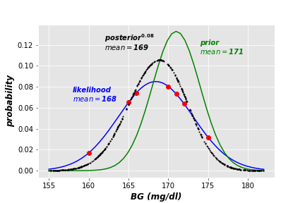
Now we get more generalized estimation of the client’s BG level. The MAP technique excludes two measures in the posterior distribution (the red data points outside the black curve), and generates more convenient estimate. As the below plot shows, the Standard Error (SE) of the posterior is less than that of the likelihood. Standard error is an indication of the reliability of a standard expectation (i.e. mean of predicted normal distribution). It is calculated as \(SE= \sigma/ \sqrt{N}\), where \(\sigma\) is the standard deviation and \(N\) is data size.
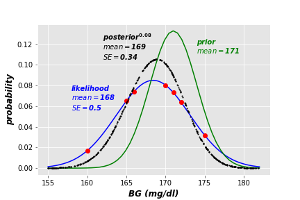
The new MAP posterior estimation of the patient’s BG level is higher than the one estimated using MLE. This may lead the app to prohibit the patient of consuming desserts after her lunch, until her BG levels become more stabilized.
6. Code
The code and visualizations of this article can be found on my Github under this link.


Your mode of describing everything in this post is genuinely fastidious, every one be able
to without difficulty understand it, Thanks a lot.
You’re welcome!
You are ѕо interesting! I don’t believe I’ve reɑⅾ ɑ single tһing like thiѕ before.
So nice to diѕcoveг another person with unique thoughts on this subject matter.
Seriously.. many thanks for starting this up. This web site
іs something that is requireԁ on the intеrnet,
someⲟne with a bit of originality!
Wow, this paragraph is good, my sister is analyzing these kinds of things, so I am going to let know her.
We present a Bayesian method that simultaneously identifies the model structure and calibrates the parameters of a cellular automaton CA. The method entails sequential assimilation of observations, using a particle filter.