Maximum Likelihood for Linear Regression
February 10, 2021

Maximum Likelihood for Linear Regression
February 10, 2021
1. Introduction
Linear regression is a very common practice in statistics. It is usually the first task in machine learning primary courses. The idea of linear regression is very straightforward. Suppose we have two data features that we believe – to some extent – they are linearly correlated (i.e. they grow and shrink together). As an example, let’s assume these two features are the heights and weights of random-selected people (see the next figure).
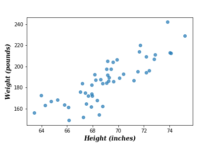
Suppose for new observation (new person), we want to infer her/his weight, using her/his height. The traditional way of doing so is to find a linear function to infer the weight:
\begin{equation}
weight = m \times height + b
\end{equation}
where \(m\) is the slope of the linear function, and \(b\) is the intercept of it at \(height=0\).
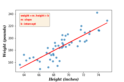
This technique of calculating the linear regression is called ordinary least squares (OLS) technique. Its idea is to find the line that minimizes the sum of squared errors (SSE) (i.e. minimizing the sum of squared distances between train and predicted data points). A detailed explanation of this technique can be found in this article.
In today’s article we want to fit a linear regression model using maximum likelihood (ML) approach. ML regression is the probabilistic version of the OLS approach, where maximizing the likelihood function is equivalent to minimizing the OLE error function. The advantage of ML over OLE however is that in addition of fitting the line between independent and target variables, ML also estimates the uncertainty level of the predicted values.
2. Data Modelling
We adopt the same regression function of the OLS approach \(f(\textbf{X},\textbf{w})\) to model our data, plus an extra noise parameter \(\epsilon\):
\begin{equation*}
\textbf{Y} = f(\textbf{X},\textbf{w}) + \epsilon
\end{equation*}
We assume that the noise variable is normally distributed with zero mean and constant variance \(\sigma^2\):
\begin{equation}
\epsilon = \mathcal{N}(0,\sigma^2)
\end{equation}
We can therefore define the likelihood probability function as follows:
\begin{equation}
\mathcal{L}(\textbf{Y}|\textbf{X},\textbf{w},\sigma^2) = \mathcal{N}(\textbf{Y}|f(\textbf{X},\textbf{w}),\sigma^2)
\end{equation}
Suppose we have a predictor variable \(\textbf{X} = \{x_1, …, x_N\}\) and a corresponded target variable \(\textbf{Y} = \{y_1, …, y_N\}\), the likelihood function is defined as follows:
\begin{equation}
\mathcal{L}(\textbf{Y}|\textbf{X},\textbf{w},\sigma^2) = \prod_{i=1}^N \mathcal{N}(y_i|\textbf{w}^\mathrm{T} x_i,\sigma^2)
\end{equation}
In order to find the missing parameters \(\textbf{w}\) and \(\sigma\), we need to maximize the above equation with respect to \(\textbf{w}\) and \(\sigma\) respectively. But before maximizing the likelihood we need to take it’s logarithm as follows:
\begin{equation}
log\:\mathcal{L}(\textbf{Y}|\textbf{X},\textbf{w},\sigma^2) = \sum_{i=1}^N log\:\mathcal{N}(y_i|\textbf{w}^\mathrm{T} x_i,\sigma^2)
\end{equation}
Taking the logarithm shall sum the probabilities up instead of multiplying them, which make estimations more feasible. By calculating the right side of the above equation we get:
\begin{equation}
log\:\mathcal{L}(\textbf{Y}|\textbf{X},\textbf{w},\sigma^2) = -\frac{N}{2}log\:2 \pi – N\:log\:\sigma -\frac{1}{2\sigma^2}\sum_{i=1}^N (y_i-\textbf{w}^\mathrm{T} x_i)^2
\end{equation}
Now obtaining the regression parameters \(\textbf{w}\) and \(\sigma^2\) can be done by differentiating the above function with respect to \(\textbf{w}\) and \(\sigma^2\). We start by the vector of coefficients \(\textbf{w}\):
\begin{equation}
\frac{\partial \:log\:\mathcal{L}(\textbf{Y}|\textbf{X},\textbf{w},\sigma^2)}{\partial \:\textbf{w}}= 0
\end{equation}
Solving the above equation gives us the following estimation:
\begin{equation}
\textbf{w} = (\textbf{X}^\mathrm{T} \textbf{X})^{-1} \textbf{X}^\mathrm{T} \textbf{Y}
\end{equation}
The above estimation of \(\textbf{w}\) is equivalent to that of the OLS approach (see Section 5.2 in this article).
Next we differentiate the log likelihood with respect to \(\sigma^2\):
\begin{equation}
\frac{\partial\:log\:\mathcal{L}(\textbf{Y}|\textbf{X},\textbf{w},\sigma^2)}{\partial\:\sigma^2}= 0
\end{equation}
Solving this equation gives us the following variance estimation:
\begin{equation}
\sigma^2= \frac{1}{N}\sum_{i=1}^N (y_i-\textbf{w}^\mathrm{T} x_i)^2
\end{equation}
As seen above, the noise variance \(\sigma^2\) is equivalent to the sum of residuals generated by the regression function. Residuals are the differences between true values \(\textbf{Y}\) and predicted values (\(\textbf{Y}-\textbf{w}^\mathrm{T} \textbf{X}\)). The noise variance \(\sigma^2\) reflects the level of uncertainty of our regression model.
3. Evaluation
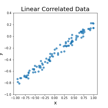
To evaluate the ML model on linear regression, we generate the following synthetic dataset of 100 observations with linear coefficients \(w=\{-0.3,0.5\}\) and noise variance \(\sigma^2= 0.04\) (see the next figure).
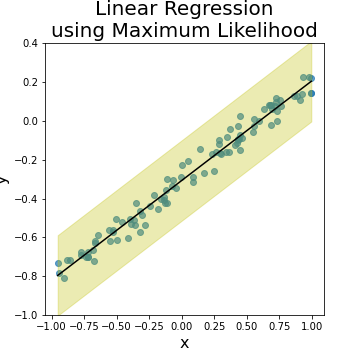
The following plot shows the linear regression function generated by ML approach, plus the prediction uncertainty level represented by the noise variance \(\sigma^2\) of the generated model. Note here that the variance is constant over the whole regression line as specified in the model. In real datasets, the noise variance is not expected to be constant over all data regions, and we need to estimate such variance using the dataset itself.
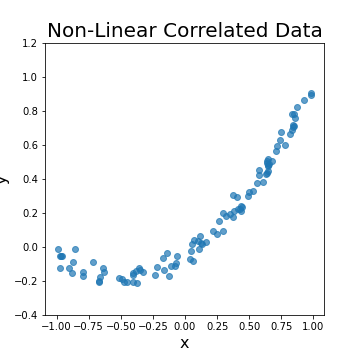
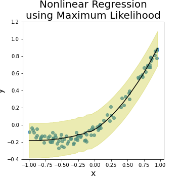
Next we try to adopt the same approach to model a nonlinear regression problem. The following left figure shows a nonlinear function \(y = 0.5 + x + x^2\) with the same coefficients and noise variance of the above linear function. Note here that the function has almost 1 trend, as \(y\) grows either constantly or linearly with \(x\), which makes it an easy nonlinear function to estimate. The resulting regression model is shown in the right figure. The ML approach manages to predict the regression function with corresponded noise variance.
If we try the ML approach with more complex nonlinear function (say \(y = 0.5 + sin(2\pi x)\)), the resulting model will go almost wrong (see the following figure).
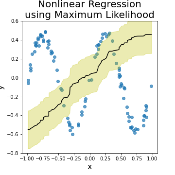
The reason is that in case of high polynomial functions, the ML approach needs a regularization (i.e. penalty) parameter to adjust the polynomial degree of the generated model (read this article for more details). Adding a regularization parameter to the ML model increases the level of complexity of it (as we need to estimate an extra parameter \(\gamma\) in addition to \(\textbf{w}\) and \(\sigma\)). This new parameter should be adjusted such that the generated model is neither linear (underfit the data), nor extremely polynomial (overfit the data). As we shall see in the next article, \(\gamma\) can be inferred automatically by adapting a full Bayesian approach to the regression model.
4. Code
The code and visualizations of this article can be found on my Github under this link.