Linear Regression
December 25, 2017
1. Idea
[watch video]
Suppose we have a set of observations represented by two variables \(x\) and \(y\). Let’s assume that our observations are group of persons, and the \(2\) variables are persons’ heights (\(x\) axis) and weights (\(y\) axis). If we plot heights and weights in a scatter plot (see below), we can easily find a kind of correlation between them (i.e. as height increase, weight increase as well, and vice versa)
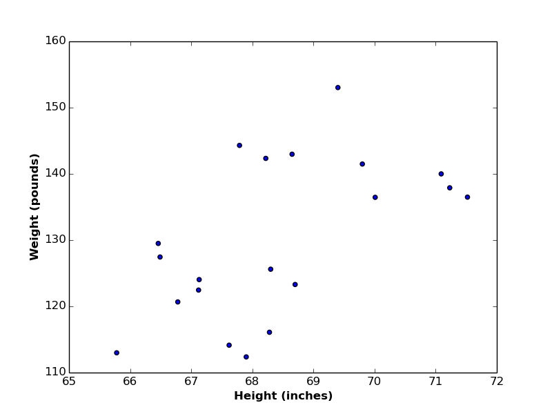
Let’s also assume that we want to find a linear relationship (i.e. linear function) between heights and weights, such that if we have the value of a new person height, we can predict her/his corresponding weight. In this case, we call variable height the independent variable or predictor, and variable weight the dependent variable or target variable.
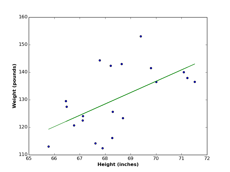
As a reminder, the linear function is defined by \(2\) coefficients (\(m\) is the slope, which reflects the change of \(y\) divided by the change of \(x\)), and \(b\) (the point at which the line intersects with \(y\) axis). In the below figure, \(m = 4.13\) and \(b = -152.43\)
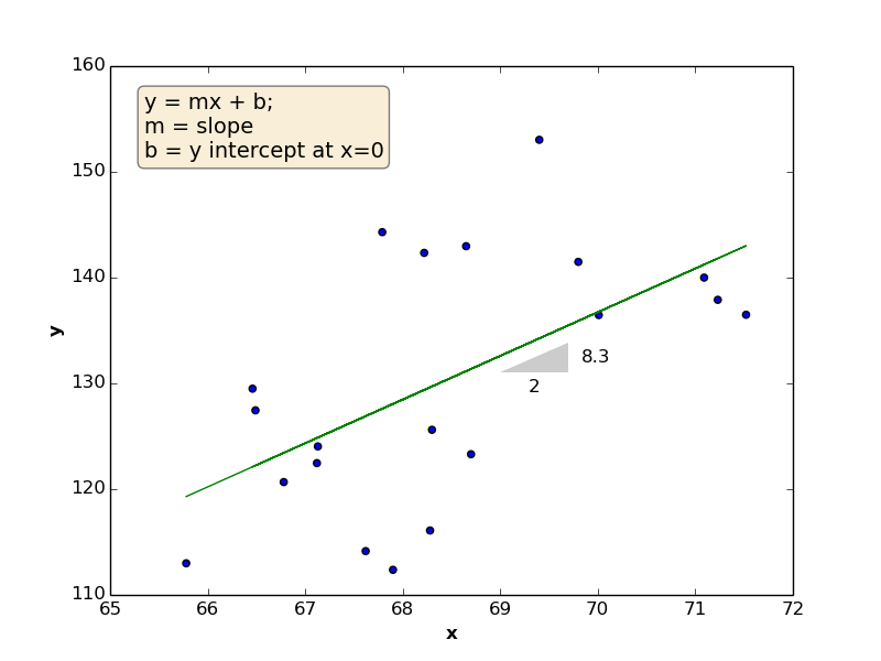
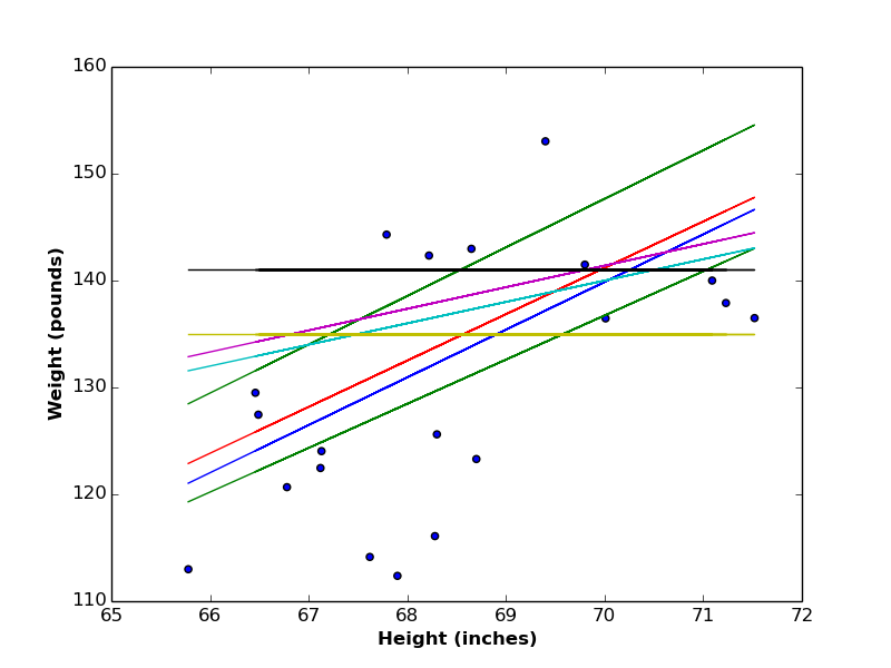
Back to our goal, we need to find a linear function between \(x\) and \(y\), but, which linear function? As you can imagine, there are endless number of lines that can represent such function (see the below figure). So the question would be, which line is the best?
Let’s go to the theory of linear regression, to be able to answer this question.
2. Theory
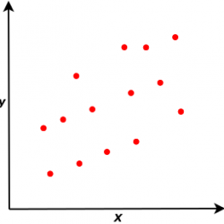
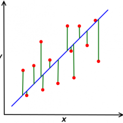
If we have a set of observations (like below left figure), the best line between variables \(x\) and \(y\) (right figure) would be the one that minimizes the distances between the observations (red dots) and their corresponded predicted values (blue linear function). This approach is called the Least Squares approach, since it minimizes the square of these distances (vertical green lines).
According to least square approach, and in order to find the best linear function between \(x\) and \(y\), we need to find a vector of coefficients \(\vec{w}\) that minimizes the following function:
\begin{equation} E(\mathbf{w}) = \frac{1}{N}\sum \limits_{i=1}^N [y^{(i)}-f(x^{(i)},\mathbf{w})]^2 \tag{1}\end{equation}
Notations:
- \(x^{(i)}\) and \(y^{(i)}\) are values of variables \(x\) and \(y\) of observation \(i\)
- \(N\) is number of observations
- \(\mathbf{w}\) is vector of coefficients to identify linear regression function
Function (1) is called error function, objective function, or cost function. In this post, a form of error function called Mean-Square-Error (MSE) is used, where squaring differences between true and predicted values allows us to consider positive and negative differences the same, and division by \(N\) allows us to compare different sizes of data using same coefficients’ values.
The function \(f(x^{(i)},\mathbf{w})\) is called linear regression function or hypothesis function, and is defined as:
\begin{equation}
f(x^{(i)},\mathbf{w}) = w_0 + w_1x^{(i)}\tag{2}
\end{equation}
where \(w_1\) is the slope and \(w_0\) is \(y\) intercept at \(x= 0\).
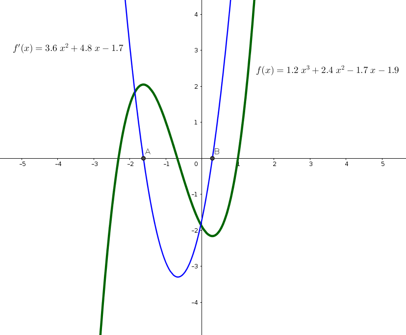
We know from Calculus, that minimizing (or maximizing) a function can be done, by equalizing it’s first derivative to zero, and solving the generated equations to find the corresponded coefficients. As an example, in the below graph, we have a function \(f(x)\) (green). If we want to find the maximum value of \(f(x)\) (Point \(A\)) or the minimum value (Point \(B\)), we compute the function’s derivative \(f'(x)\) (blue), and find the points where \(f'(x)\) intersects with \(x\) axis.
Let’s try to differentiate Equation (1) with respect to \(\mathbf{w}\) and find the values of \(w_0\) and \(w_1\).
compute \(w_0\) (\(y\) intercept at \(x=0\))
\begin{equation}
\frac{\partial E(\mathbf{w})}{\partial w_0}= \frac{1}{N} \sum\limits_{i=1}^N \frac{\partial [y^{(i)} – (w_0 + w_1 x^{(i)})]^2}{\partial w_0}\tag{3}
\end{equation}
\begin{equation}
\frac{\partial E(\mathbf{w})}{\partial w_0}= \frac{1}{N} \sum\limits_{i=1}^N \frac{\partial [{y^{(i)}}^2 -2y^{(i)}(w_0 + w_1 x^{(i)}) + (w_0 + w_1 x^{(i)})^2 ]}{\partial w_0}\tag{4}
\end{equation}
\begin{equation}
\frac{\partial E(\mathbf{w})}{\partial w_0}= \frac{1}{N} \sum\limits_{i=1}^N \frac{\partial [{y^{(i)}}^2 – 2w_0 y^{(i)} – 2 w_1 x^{(i)} y^{(i)} + w_0^2 + 2w_0 w_1 x^{(i)} + w_1^2 {x^{(i)}}^2] }{\partial w_0}\tag{5}
\end{equation}
\begin{equation}
\frac{\partial E(\mathbf{w})}{\partial w_0}= \frac{1}{N} \sum\limits_{i=1}^N -2 y^{(i)} +2 w_0 + 2 w_1 x^{(i)}\tag{6}
\end{equation}
\begin{equation}
\frac{\partial E(\mathbf{w})}{\partial w_0}= \frac{-2}{N} \sum\limits_{i=1}^N y^{(i)} – (w_0 + w_1 x^{(i)}) \tag{7}
\end{equation}
compute \(w_1\) (slope)
for this part, we will differentiate Equation (5) with respect to \(w_1\), as follows:
\begin{equation}
\frac{\partial E(\mathbf{w})}{\partial w_1}= \frac{1}{N} \sum\limits_{i=1}^N \frac{\partial [{y^{(i)}}^2 – 2w_0 y^{(i)} – 2 w_1 x^{(i)} y^{(i)} + w_0^2 + 2w_0 w_1 x^{(i)} + w_1^2 {x^{(i)}}^2] }{\partial w_1}\tag{8}
\end{equation}
\begin{equation}
\frac{\partial E(\mathbf{w})}{\partial w_1}= \frac{1}{N} \sum\limits_{i=1}^N -2 x^{(i)} y^{(i)} +2 w_0 x^{(i)} + 2 w_1 {x^{(i)}}^2\tag{9}
\end{equation}
\begin{equation}
\frac{\partial E(\mathbf{w})}{\partial w_1}= \frac{-2}{N} \sum\limits_{i=1}^N x^{(i)}[y^{(i)} – (w_0 + w_1 x^{(i)})] \tag{10}\end{equation}
Please note, that the only difference between equations (7) and (10), is that when we differentiate the error function with respect to the second coefficient \(w_1\), we multiply the right side inside the sigma by \(x^{(i)}\).
Now, we put both (7) and (10) equations to zero:
\begin{equation}
\frac{-2}{N} \sum\limits_{i=1}^N y^{(i)} – (w_0 + w_1 x^{(i)}) = 0\tag{11}
\end{equation}
\begin{equation}
\frac{-2}{N} \sum\limits_{i=1}^N x^{(i)}[y^{(i)} – (w_0 + w_1 x^{(i)})] = 0\tag{12}
\end{equation}
There are two ways to solve this equations system and obtain \(\mathbf{w}\): a closed form approach, and the gradient descent algorithm.
3. Closed Form Approach
[watch video]
Let us remove the \(N\) fraction and re-order equations (11), (12):
\begin{equation}
\sum\limits_{i=1}^N y^{(i)} = w_0 N + w_1 \sum\limits_{i=1}^N x^{(i)}\tag{13}
\end{equation}
\begin{equation}
\sum\limits_{i=1}^N x^{(i)}y^{(i)} = w_0 \sum\limits_{i=1}^N x^{(i)} + w_1 \sum\limits_{i=1}^N {x^{(i)}}^2\tag{14}
\end{equation}
Now, we have 2 equations in 2 missing variables, which can be solved if we re-write equations (13) and (14) in matrix form:
\begin{gather}
\begin{bmatrix} \sum\limits_{i=1}^N y^{(i)} \\ \sum\limits_{i=1}^N x^{(i)}y^{(i)} \end{bmatrix}
=
\begin{bmatrix} w_0 \\ w_1 \end{bmatrix}
\begin{bmatrix}
N &
\sum\limits_{i=1}^N x^{(i)} \\
\sum\limits_{i=1}^N x^{(i)} &
\sum\limits_{i=1}^N {x^{(i)}}^2
\end{bmatrix}\tag{15}
\end{gather}
which simulates the form:
\begin{equation}
\mathbf{B} = \mathbf{wA}\tag{16}
\end{equation}
then the vector \(\mathbf{w}\) is computed as:
\begin{equation}
\mathbf{w} = \mathbf{A}^{-1} \mathbf{B}\tag{17}
\end{equation}
4. Gradient Descent Algorithm
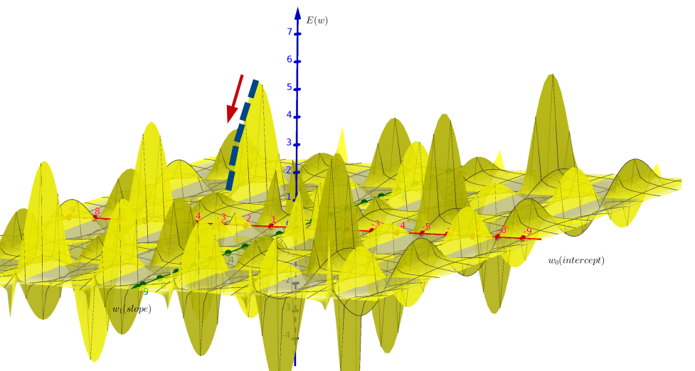
We can imagine the gradient descent algorithm for linear regression as a \(3\)d graph (see below). We start at random values of \(\mathbf{w}\), compute the corresponded error function \(E(\mathbf{w})\), and iteratively updating \(\mathbf{w}\) in the direction of lowering \(E(\mathbf{w})\), until either \(\nabla E(\mathbf{w})= 0\), or a satisfied converge is reached.
Gradient descent algorithm (listed below) require three input parameters: the cost function \(E(\mathbf{w})\) to be differentiated, initial values of linear coefficients vector \(\mathbf{w}\), and a third parameter called the learning rate. The role of learning rate is to control the algorithm speed while minimizing the error function. On the one hand, if learning rate take high values, the algorithm will converge quickly, but it can fall into a local minima. On the other hand, if learning rate is small, the algorithm may take considerable running time to converge. Different values of \(\eta\) should be tested to select the most probable value for data in hand.
Algorithm1 GradientDescent(\(E(\mathbf{w}),\mathbf{w},\eta\))
- Input:
- \(E(\mathbf{w})\): cost function
- \(\mathbf{w}\): initial values of coefficients vector
- \(\eta\): learning rate
- Output:
- \(\mathbf{w}\): updated values of coefficients vector
- Procedure:
- repeat
- \(w_p=w_p – \eta \frac{\partial E(\mathbf{w})}{\partial w_p}, \forall w_p \in \mathbf{w}\)
- until \(\nabla E(\mathbf{w})= 0\)
- return \(\mathbf{w}\)
Coefficients (\(w_p\)) in the gradient descent algorithm are updated as follows:
\begin{equation}
w_0= w_0 – \eta \frac{-2}{N} \sum\limits_{i=1}^N y^{(i)} – (w_0 + w_1 x^{(i)}) \tag{18}
\end{equation}
\begin{equation}
w_1= w_1 – \eta \frac{-2}{N} \sum\limits_{i=1}^N [y^{(i)} – (w_0 + w_1 x^{(i)})] x^{(i)}\tag{19}
\end{equation}
5. Multivariate Linear Regression
In the above discussion, we considered one independent variable \(x\) (heights) to learn from. Now, suppose that we have multiple independent variables \(\mathbf{x}=[x_1, x_2 …,x_M]\). As an example, let’s assume we have heights, ages and blood pressures of a group of persons, and we want to use all these predictors to predict the weight variable. In this case, our linear regression function (equation 2), will be expanded to:
\begin{equation}
f(\mathbf{x}^{(i)},\mathbf{w}) = w_0 x_0^{(i)} + w_1 x_1^{(i)} + w_2 x_2^{(i)} + … + w_M x_M^{(i)}\tag{20}
\end{equation}
or in more compact form:
\begin{equation}
f(\mathbf{x}^{(i)},\mathbf{w}) = \sum\limits_{j=0}^M w_j x_j^{(i)}\tag{21}
\end{equation}
Notations:
\(x_j^{(i)}\) is the value of independent variable \(x_j\) at observation \(i\)
\(M\) is number of independent variables (i.e. predictors)
\(\mathbf{w}\) is vector of coefficients to identify linear regression function
5.1 Computing Coefficients Vector \(\mathbf{w}\)
In order to compute \(\mathbf{w}\), we re-formulate equations (7) and (10) in one equation as follows:
\begin{gather}
\begin{aligned}
\frac{\partial E(\mathbf{w})}{\partial w_j}= \frac{-2}{N} \sum\limits_{i=1}^N x_j^{(i)}[y^{(i)} – f(\mathbf{x}^{(i)},\mathbf{w})],
\\
\forall j \in [0:M], x_0^{(i)} = 1
\end{aligned}\tag{22}
\end{gather}
As an example, suppose we have \(2\) independent variables (i.e. \(M=2\)). This means we need to compute \(3\) coefficients \(w_0\), \(w_1\) and \(w_2\). Our regression (i.e. hypothesis) function would be:
\begin{equation}
f(\mathbf{x}^{(i)},\mathbf{w}) = w_0 x_0^{(i)} + w_1 x_1^{(i)} + w_2 x_2^{(i)}\tag{23}
\end{equation}
by setting \(x_0^{(i)} = 1\), the equation will be:
\begin{equation}
f(\mathbf{x}^{(i)},\mathbf{w}) = w_0 + w_1 x_1^{(i)} + w_2 x_2^{(i)}\tag{24}
\end{equation}
The corresponded error function derivatives will be:
\begin{equation}
\frac{\partial E(\mathbf{w})}{\partial \mathbf{w}}= \frac{-2}{N} \sum\limits_{i=1}^N x_j^{(i)}[y^{(i)} – (w_0 + w_1 x_1^{(i)} + w_2 x_2^{(i)})]\tag{25}
\end{equation}
5.2 Closed Form Approach
In order to apply the closed-form approach on multivariate linear regression, we build two matrices: the following \(N \times (M+1)\) matrix \(\mathbf{X}\) represents the matrix of independent variables. please note that the first column set to 1’s is corresponded to \(x_0^{(i)}\) is equation (22).
\begin{gather}
\mathbf{X}
= \begin{bmatrix}
1 & x_1^{(1)} & x_2^{(1)} & … & & x_M^{(1)} \\\\
1 & x_1^{(2)} & x_2^{(2)} & … & & x_M^{(2)} \\\\
\vdots \\\\
1 & x_1^{(N)} & x_2^{(N)} & … & & x_M^{(N)}
\end{bmatrix}
\end{gather}
and the following \(N \times 1\) matrix \(\mathbf{Y}\) represents the dependent variable \(y\):
\begin{gather}
\mathbf{Y}
= \begin{bmatrix}
y^{(1)} \\\\
y^{(2)} \\\\
\vdots \\\\
y^{(N)}
\end{bmatrix}
\end{gather}
After building these two matrices, the vector of coefficients \(\mathbf{w}\) is calculated as:
\begin{equation}
\mathbf{w} = (\mathbf{X}^T \mathbf{X})^{-1} \mathbf{X}^T \mathbf{Y}\tag{26}
\end{equation}
5.3 Gradient Descent Algorithm
The gradient descent algorithm for 1 independent variable is still valid for multi independent variables. The sole change will be in definitions of error function derivatives according to equation (22). As an example, the following updates are valid in the case of 2 independent variables:
\begin{equation}
w_0= w_0 – \eta\frac{-2}{N} \sum\limits_{i=1}^N y^{(i)} – (w_0 + w_1 x_1^{(i)} + w_2 x_2^{(i)})
\end{equation}
\begin{equation}
w_1= w_1 – \eta\frac{-2}{N} \sum\limits_{i=1}^N x_1^{(i)} [y^{(i)} – (w_0 + w_1 x_1^{(i)} + w_2 x_2^{(i)})]
\end{equation}
\begin{equation}
w_2= w_2 – \eta\frac{-2}{N} \sum\limits_{i=1}^N x_2^{(i)} [y^{(i)} – (w_0 + w_1 x_1^{(i)} + w_2 x_2^{(i)})]
\end{equation}
Please note that in order to compute each coefficient \(w_j\), you need the previous values for all other coefficients, including \(w_j\).
6. Closed Form or Gradient Descent?
There is no doubt that closed form solution is the most convenient way to calculate the vector of coefficients \(\mathbf{w}\), as long as your computer can compute matrix \((\mathbf{X}^T \mathbf{X})^{-1}\) in feasible time. Please note that this is a \(M \times M\) matrix, which can take long running time if number of predictors \(M\) is large. In addition, gradient descent algorithm is efficient for data with large number of predictors \(M\), but you must take care of selecting suitable value for learning rate \(\eta\).
7. Implementation in Python
You can find python implementations of the above algorithms on my GitHub.


