Bayes Theory and Its Facts
January 6, 2021

Bayes Theory and Its Facts
January 6, 2021
- Example and Bayesian Treatment
- Interpretation
- New evidences do not neglect or overwrite the prior, but update it
- Each new evidence can drastically change the final estimation
- Likelihood is NOT a probability of events, it’s a probability of hypotheses!
- Likelihoods are meaningless, unless compared to each other!
- Marginal likelihood is constant over all hypotheses!
- Proof of Bayes Theorem
1. Example and Bayesian Treatment
” John is software engineer with 15+ years of technical experiences in IT. He applied to the CTO position in a startup company. In the final interview, and among a short list of 5 applicants , John was double qualified than the other four candidates. Do you think that John got the job? “
If I am willing to guess, I will assume that John definitely got the job, says with 90% chance. I think also that you agree with me, do you? Based on the available information, John has over-performed all other applicants in the last round of interviews. Accordingly, he is the most likely to get the job. But does Bayes’ Theory shares us the same opinion? Let us see how Bayes’ Theorem guesses the answer!
The first step in Bayes’ Theory is to estimate the probability that John got the job. This assumption is usually called the hypothesis (H). As all applicants in the short list have equal opportunity to get the job, John – as well as the other four – has equal probability of 1/5 (or 20%) to get the job. This estimation is called the prior and can be written as:
\begin{equation}
P(H) = \frac{1}{5} = 20\%
\end{equation}
There is another piece of information; that is, John is double qualified than the other four applicants after the final evaluation. This piece of information is called the evidence (E), and it is the information piece that should update our prior believe (John got the job). The goal now is to calculate the probability that John got the job (i.e. P(H)), given the fact that John was double-qualified for the job than all other applicants (i.e. E). This probability is called the posterior and it is mathematically written as P(H|E).
But how can we update our hypothesis (H) using the evidence (E)? Here comes Bayes’ Theorem into the picture. Bayes’ Theory binds the prior and the posterior by a third component called the likelihood. The likelihood is nothing but the opposite conditional probability to the posterior (i.e. P(E|H)) or the probability that John was double-qualified than all other applicants, given that John got the Job.
In order to calculate the likelihood of our example, we need to quantify our evidence with numbers. Suppose the last interview round includes an evaluation sheet of 10 points. In this evaluation sheet John got 8/10 while each other applicant got only 4/10. We can translate these ratios into probabilities as follows:
\begin{equation*}
P(\textit{John was double-qualified $|$ John got the job}) = P(E|H) = 0.8
\end{equation*}
\begin{equation*}
P(\textit{John was double-qualified $|$ John did not get the job}) = P(E|\neg H) = 0.4
\end{equation*}
Now we can write Bayes’ Theorem as:
\begin{equation*}
Posterior \propto Likelihood \times Prior
\end{equation*}
or:
\begin{equation*}
P(H|E) \propto P(E|H) \times P(H)
\end{equation*}
Note that both sides are proportional to each other! in order to equalize them, we need to normalize the right side by using the marginal probability. Marginal probability is the total probability of seeing the evidence E, whether the hypothesis H holds or not. It is calculated as follows:
\begin{equation*}
\begin{split}
\textit{marginal prob.} & = P(E \cap H) + P(E \cap\neg H)\\
& = P(E|H) \times P(H) + P(E|\neg H) \times P(\neg H)
\end{split}
\end{equation*}
Now we can re-write Bayes’ Theorem as:
\begin{equation*}
P(H|E) =\dfrac{P(E|H) \times P(H)}{P(E|H) \times P(H) + P(E|\neg H) \times P(\neg H)}
\end{equation*}
For simplicity and symmetry, the denominator is usually written as P(E):
\begin{equation*}
{\boxed{P(H|E) =\dfrac{P(E|H) \times P(H)}{P(E)} } }
\end{equation*}
Let’s plug in our numbers and calculate the posterior given the above data:
\begin{equation}
\begin{split}
P(H|E) & =\dfrac{P(E|H) \times P(H)}{P(E|H) \times P(H) + P(E|\neg H) \times P(\neg H)}\\\\
& = \frac{0.8 \times 0.2}{0.8 \times 0.2 + 0.4 \times 0.8} = \frac{0.16}{0.16+0.32} = \frac{0.16}{0.48} \\\\
&= \frac{1}{3} \approx 33\%
\end{split}
\end{equation}
The above result says that according to Bayes’ Theorem, John has 33% chance to be the CTO, given that he double-qualified all other applicants! Does this result make sense to you?
2. Interpretation
The easiest way to understand Bayes’ Rule is to think of it as a function of time \(f(T)\). At the first moment (say \(T_0\)), we build our hypothesis (prior). At each next moment, we update our prior using Bayes’ equation. In our example, we can consider the first moment \(T_0\) is when the startup creates the short list of the five candidates. At this point, we build our prior hypothesis as follows:
\begin{equation*}
P(\textit{John got the job},T_0) = \frac{1}{5} = P(\textit{another candidate got the job},T_0)
\end{equation*}
At time point \(T_1\), the startup has interviewed the five candidates, and it turns out that John is double-performed than the other 4 candidates. Now we update our prior as follows:
\begin{equation*}
P(\textit{John got the job},T_1) = 2 \times P(\textit{another candidate got the job},T_1)
\end{equation*}
Now the probabilities must change to meet the new evidence. To calculate the new probabilities, we assign each candidate (other than John) a probability of \(\frac{1}{6}\), such that:
\begin{equation*}
P(\textit{another candidate got the job},T_1) = \frac{1}{6}\approx 17\%
\end{equation*}
\begin{equation*}
P(\textit{John didn’t get the job},T_1) = 4\times\frac{1}{6} = \frac{2}{3}\approx 76\%
\end{equation*}
\begin{equation*}
\begin{split}
P(\textit{John got the job},T_1) & = 1 – \frac{2}{3}\\
& = \frac{1}{3}\approx 33\%\\
& = 2 \times P(\textit{another candidate got the job},T_1)
\end{split}
\end{equation*}
This is the same result we calculated using Bayes’ Theorem. After updating our prior with the new evidence, the probability that John got the job increased from 20% to 33%, and doubled the probability that another candidate got the job (around 17%). The result – however – did not neglect the fact that John still has four qualified competitors, and the sum of probabilities of those competitors should be considered in the final evaluation. This leads us to the first fact of Bayes’ Theorem.
3. Fact #1: New evidences do not neglect or overwrite the prior, but update It
Bayes’ Theorem does not working like human minds. While human minds usually overwrite information and highlight the most significant pieces of it, Bayes’ Theory has a strong memory that cumulate information over time and update its outputs afterwards. In our example, even if John is 3 times more qualified than other candidates in the final interview, his chances to get the job according to Bayes’ Rule is around 43%. If he is 4 times more qualified than others, his chance shall not exceed 50%. As you notice, Bayes’ Rule increases John chances according to his achievements in the interview (the evidence) without ignoring the fact that he is one of 5 qualified candidates for the job.
4. Fact #2: Each new evidence can drastically change the final estimation
This fact seems to contradict the first one, but it holds in all cases. In order to illustrate this fact, we add an update to the above example:
” … while the startup founders were deciding about the CTO position, they received a feedback from a big investor who was ready to fund their startup. The investor asked however, that the company CTO must be 5 days a week in the company’ office. The founders asked John to relocate to their city, but John refused their demand for social reasons. He offered instead to be in the office only 1 day/week, and the rest of the week working from home. The other 4 candidates were ready to work full time from office. After this update, what is the chance that John got the job? “
In this update, a new evidence (say \(E_2\)) has been added to the problem. To plug it into the Bayes’ Rule, we need to quantify the new information in both likelihood and marginal probability. Let’s start with the likelihood:
\begin{equation}
P(\textit{CTO work from office $|$ John got the job}) = \frac{1}{5} = P(E_2|H)\\\\
P(\textit{CTO work from office $|$ John didn’t get the job}) = 1 = P(E_2|\neg H)
\end{equation}
And the marginal probability:
\begin{equation*}
\begin{split}
& P(E_1,E_2|H)) \times P(H) + P(E_1,E_2|\neg H)) \times P(\neg H) =\\
& (0.8 \times 0.2 \times 0.2) + (0.4 \times 1 \times 0.8) = 0.352
\end{split}
\end{equation*}
Now we update the posterior as follows:
\begin{equation*}
\begin{split}
P(H|E_1,E_2) & = \frac{P(E_1,E_2|H) \times P(H)}{P(E_1,E_2|H) \times P(H) + P(E_1,E_2|\neg H) \times P(\neg H)}\\\\
& = \frac{0.8 \times 0.2 \times 0.2}{0.352} = 0.09 = 9\%
\end{split}
\end{equation*}
As the result shows, the new evidence has dropped John chance to get the job from 33% down to 9%. This gives us an example of how much a new evidence can dramatically change a Bayesian estimation.
5. Fact #3 Likelihood is NOT a probability of events, it’s a probability of hypotheses!
The Likelihood is the basic – yet the most ambiguous part – of Bayes’ Rule. Many people treat likelihoods as probability values, and they get confused when discover that it does not meet probability postulations. The fact is that likelihood is a special type of probability called probability of hypotheses or probability of probabilities.
This means the likelihood calculations are build upon hypotheses, not upon data or measurements (at least within the focus of this article). Because the impeded hypotheses are not disjoint and exhaustive probabilities, the generated likelihoods do not follow the postulations of common (i.e. event) probabilities. For instance, the likelihood and its complement(s) must not sum up to 1. In addition, likelihoods can not be interpreted as informative ratios.
Back to John’s case, we saw that after the last interview it turns out that John was double qualified than all other candidates. We express this likelihood as follows:
\begin{equation}
P(\textit{John was double-qualified $|$ John got the job}) = P(E|H) = 0.8\\ \\
P(\textit{John was double-qualified $|$ John did not get the job}) = P(E|\neg H) = 0.4
\end{equation}
As you see, the likelihood \(P(E|H)\) and its complement \(P(E|\neg H)\) do not sum up to 1. This makes sense; like for example if a number of students took an exam, it is very unlikely that the sum of their marks equals exactly the full mark of the exam. Moreover, the likelihood values mentioned above can not be exclusively interpreted as percentages, as these values are just proportional to each other. I assume here that the ratio is 0.8:0.4. You may assume it’s 1:0.5 or 0.6:0.3. As all these ratios are equivalent to 2:1, plugging any of them leads to the same posterior estimation.
6. Fact #4 Likelihoods are meaningless, unless compared to each other!
There are endless ways of estimating the probability of a hypothesis. Accordingly, no body can be 100% sure of his, or others’ estimations of a given question. For example, if you give a golden ring to 12 jewelers, and ask each of them to estimate the ring weight by hand. Each one shall give an approximate value according to her/his experience and hand sensitivity. Let’s say their estimations (in grams) are \(\{4,3.9,3.85,3.8,4,3.9,3.9,3.85,3.9,3.85,3.95,3.9\}\).
If we want to evaluate these estimations, we can’t do this selectively, as all estimations have the same degree of uncertainty. The solution is to measure the likelihood of each weight, and the weight with maximum likelihood estimation gains the lowest degree of uncertainty (or highest reliability).
\begin{equation*}
\begin{split}
\textit{Likelihood}(3.8)= \frac{1}{12}\\
\textit{Likelihood}(3.85)= \frac{3}{12}\\
\textit{Likelihood}(3.9)= \frac{5}{12}\\
\textit{Likelihood}(3.95)= \frac{1}{12}\\
\textit{Likelihood}(4)= \frac{2}{12}
\end{split}
\end{equation*}
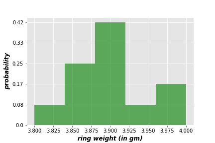
From this simple evaluation, we find that 3.9 is the weight with maximum likelihood, and it gains a probability of 42%. This technique is know as the Maximum Likelihood Estimation (MLE), which is widely used in data analysis.
In addition to MLE, we can assign a range of reliability to the MLE analysis. In our example, the following graph shows that 90% of data lies between 3.87 and 3.93.
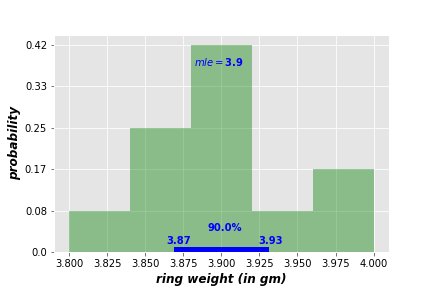
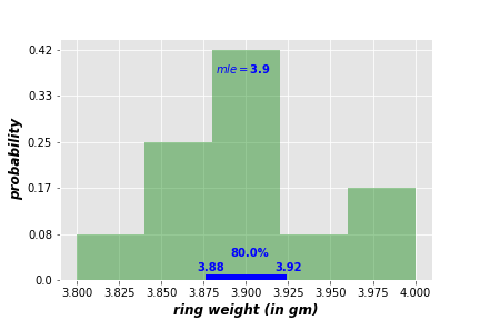
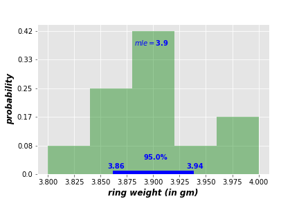
This range is called the Credible Interval CI (or Highest Posterior Density HPD), and it indicates that 90% of the hypotheses are more likely to be between 3.87 and 3.93. You can expand or shrink the credible interval to meet your analysis requirements. Following are credible intervals of 80% (left) and 95% (right).
7. Fact #5 Marginal likelihood is constant over all hypotheses!
I mentioned earlier that marginal likelihood is just a normalizer that ensures the generated posterior is a valid ratio. Because marginal likelihood is data-independent, it has no influence on the posterior estimations. Let’s have a look at the posterior estimation of a hypothesis \(H\) given an evidence \(E\):
\begin{equation*}
P(H|E) =\dfrac{P(E|H) \times P(H)}{P(E|H) \times P(H) + P(E|\neg H) \times P(\neg H)}
\end{equation*}
By replacing hypothesis \(H\) with it’s complement \(\neg H\), the posterior is calculated as follows:
\begin{equation*}
P(\neg H|E) =\dfrac{P(E|\neg H) \times P(\neg H)}{P(E|H) \times P(H) + P(E|\neg H) \times P(\neg H)}
\end{equation*}
Note here that the denominator on the right side has not changed, which emphasizes the neutrality of marginal likelihood over different hypotheses. This fact has a lot of consequences in real life applications. For instance, if you decide to apply Bayes Rule in its simplest form (i.e. MLE), you don’t need (and you can’t) calculate the marginal likelihood, due to the absence of prior probability \(P(H)\). If you build a Naive Bayes Classifier, you also don’t need to compute marginal likelihood, because it has no influence on the classification results.
8. Proof of Bayes Theorem
As an appendix to this article, I want to give a simple proof of Bayes Theorem, which is very simple and straightforward. Bayes Rule could be easily inferred using joint probability axiom of 2 independent events \(A\) and \(B\):
\begin{equation*}
P(A \cap B) = P(A|B) \times P(B)
\end{equation*}
In the same way, we can define the joint probability of \(B\) and \(A\):
\begin{equation*}
P(B \cap A) = P(B|A) \times P(A)
\end{equation*}
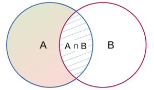
As joint probabilities are interchangeable (i.e. \(P(A \cap B)=P(B \cap A)\)), we can also write that:
\begin{equation*}
P(A|B) \times P(B) = P(B|A) \times P(A)
\end{equation*}
which gives us the Bayes Theorem:
\begin{equation*}
P(A|B) = \frac{P(B|A) \times P(A)}{P(B)}
\end{equation*}