Logistic Regression
January 24, 2018
1. Idea
1.1 Quantitative and Categorical variables
[watch video]
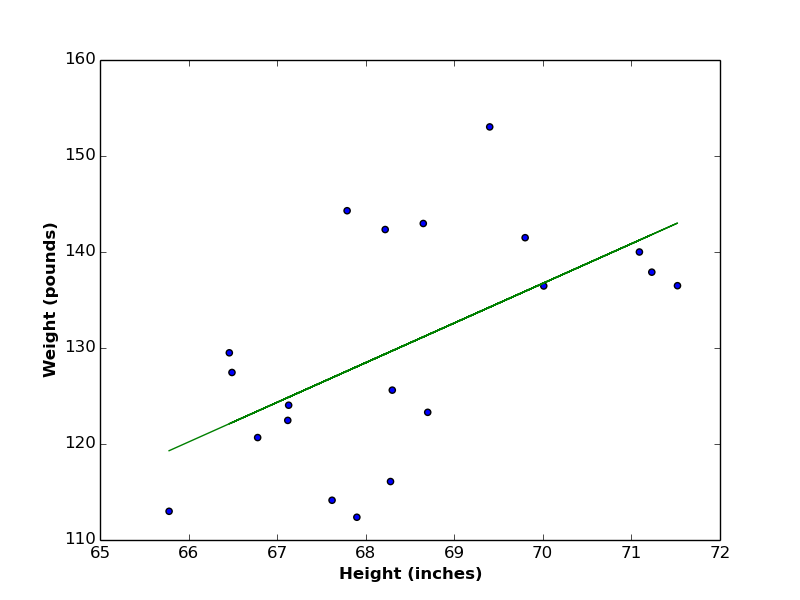
In the linear regression article, we worked with quantitative (continuous) variables like persons’ heights and weights, where each variable takes numerical values. We managed to find a linear relationship between such variables.
There exists another type of variables, called discrete (or categorical) variables. Values of discrete variables have finite number of states (or classes) that represent the whole variable. Examples of categorical variables include (gender {Male, Female}, switch power {ON, OFF}, test result {Pass,Fail}), and so on. In the following table of persons’ data, two continuous variables are listed (Height and Weight), along with one categorical variable (Gender). \begin{array}{|c|c|c|c|c|c|}
\hline Height & 73.84 & 68.78 & 58.21 & 63.03 & 71.81 \\\hline
\hline Weight & 241.89 & 162.31 & 101.75 & 126.73 & 205.92 \\\hline
\hline Gender & Male & Male & Female & Female & Male \\\hline
\end{array}
1.2 Regression vs. Classification
If the feature you want to predict (i.e. your target variable) is continuous, the prediction method is usually called regression, while if your target variable is categorical, the prediction method is called classification. However, the classification method discussed in this post is called logistic regression for historical reasons.
1.3 Preprocessing (Encoding)
A required preprocessing step for categorical variables is to encode them (i.e. to convert each class to a unique numerical value) to be able to apply calculations on them. In the above example of persons’ data, the class “Female” is encoded to 0, while the class “Male” is encoded to 1 (see the following table).
\begin{array}{|c|c|c|c|c|c|}
\hline Height & 73.84 & 68.78 & 58.21 & 63.03 & 71.81 \\\hline
\hline Weight & 241.89 & 162.31 & 101.75 & 126.73 & 205.92 \\\hline
\hline Gender & 1 & 1 & 0 & 0 & 1 \\\hline
\end{array}
2. Theory
2.1 Classification Function Requirements
As a first step, let us visualize both types of variables in the following blots:
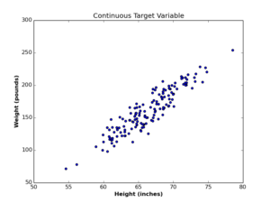
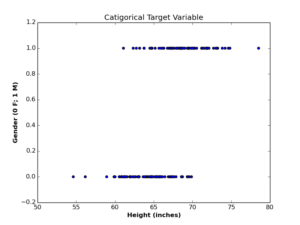
In the case of continuous variables (left plot), we managed to find a linear function that represent the relationship between Height and Weight. In the case of the categorical (Gender) variable (right plot), the situation is different, as we want a hypothesis function to generate values in range [0,1], in order to be able to round it to either classes. In other words, we want the output to be interpreted as a probability. If the probabilistic outcome of classification function is \(\geq 0.5\), we consider the gender is more likely to be 1 (or “Male”). If the outcome \(< 0.5\), we consider the gender is more likely to be 0 (or “Female”).
2.2 Linear Model
Let us begin with the linear model, and see if it fulfills our classification requirement. The following plot contains the linear regression function between Height and Gender variables.
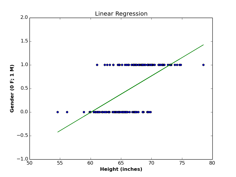
The regression line above is defined by:
\begin{equation}
P(gender=1) = 0.08\times height -4.65\tag{1}
\end{equation}
We use \(P\) here to refer to a probability function, and the probability measured here is the probability that the outcome is \(1\). In case of binary classification, this implicitly means that \(P(gender=0) = 1 – P(gender=1)\).
As an example, if we substitute the \(height\) variable with value \(65\), we will get:
\begin{equation}
P(gender=1) = 0.08\times 65 -4.65 = 0.55
\end{equation}
This means that a person with \(65\) inches height has a \(55\%\) chance to be a Male, and \(45\%\) chance to be a Female. Which makes sense, since the outcome is a probability value between \(0\) and \(1\). What if we try another \(height\) value (say \(57\))?
\begin{equation}
P(gender=1) = 0.08\times 57 -4.65 = -0.09
\end{equation}
As you can see, the linear model here generates unacceptable probabilistic value, since the probability value must be positive. Lets try out another \(height\) value (say \(75\)):
\begin{equation}
P(gender=1) = 0.08\times 75 -4.65 = 1.33
\end{equation}
Again, the linear model generates unacceptable probability value, since valid probabilities must be \(\leq 1\). Therefore, we conclude that linear model is not suitable for predicting discrete variables.
2.3 Heaviside (Step) Model
Another idea would be to use linear model, with considering every outcome \(< 0\) as \(0\), and every outcome \(> 1\) as \(1\). This model is represented by the following graph.
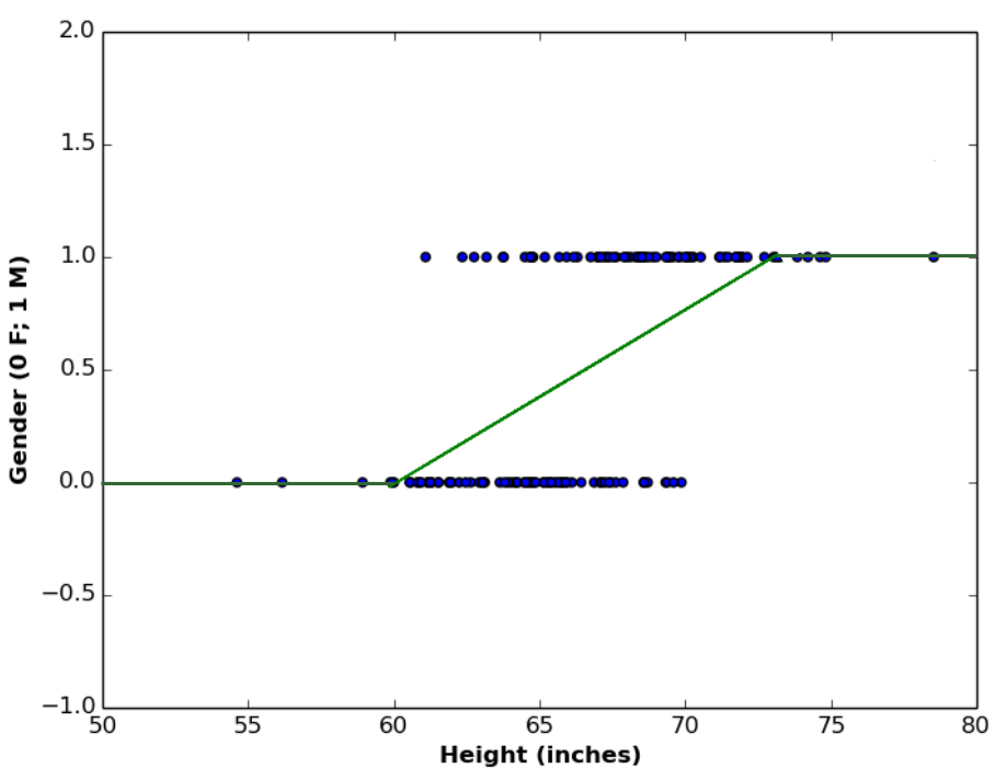
The above plotted function is called heaviside function or step function, which is a type of a family of functions called piecewise functions. It is called so because it has multiple definitions, depending on the domain it is defined for.
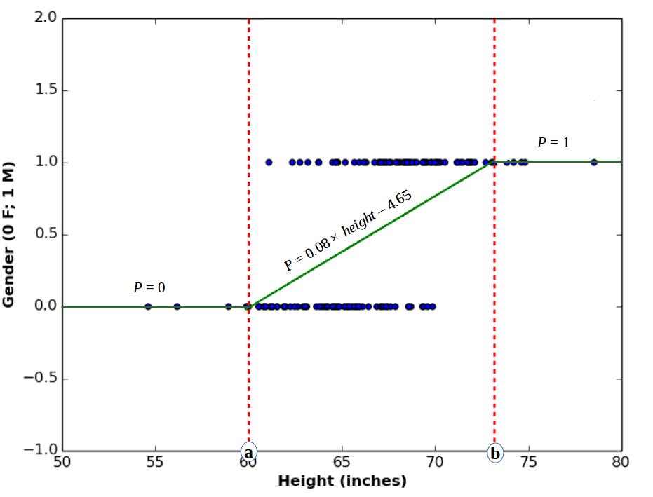
\begin{equation}
P(gender=1) = \begin{cases}
0, & \mbox{if } height\leq a \\
0.08\times height -4.65, & \mbox{if } a < height < b \\
1, & \mbox{if } height\geq b
\end{cases}\tag{2}
\end{equation}
Although this function satisfies the probabilistic outcome of \(P\), it suffers from another drawback, that is, it is not smooth. By smoothness we mean, that the function should be differentiable everywhere over its domain. Obviously, this is not the case with the step function shown above, since it is equal to constant values in ranges \(height\leq a\) and \(height\geq b\), which makes it’s first derivative over these sub-domains equal to \(0\).
Smoothness is an important condition in any regression or classification function we select, since we usually need to differentiate the cost function to minimize (or maximize) it. Therefore, we conclude that step functions are also not suitable for classification problems.
2.4 Logistic Model
The most suitable function for our classification problem is the sigmoid (or logistic) function, and it looks like the function below:
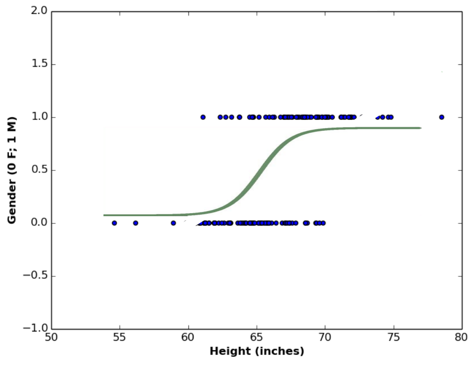
Logistic function satisfies all conditions we need for a classification problem. It is probabilistic (i.e. in range \([0,1]\)), continuous (i.e. defined in every point of its domain), and smooth (i.e. differentiable over every point of its domain). The logistic function is defined as follows:
\begin{equation}
P(y^{(i)}=1) = \frac{1}{1+e^{-f(x^{(i)},\mathbf{w})}}\tag{3}
\end{equation}
where \(f(x^{(i)},\mathbf{w})\) is a linear function defined as:
\begin{equation}
f(x^{(i)},\mathbf{w}) = w_0 + w_1 x^{(i)}_1 + w_2 x^{(i)}_2 + … + w_k x^{(i)}_k\tag{4}
\end{equation}
where \(k\) refers to number of predictors. We can re-write Equation (4) in vector form as follows:
\begin{equation}
f(\mathbf{x},\mathbf{w}) = \begin{bmatrix}
w_0 \\
w_1 \\
w_2 \\
\vdots \\
w_k \\
\end{bmatrix}
\times
\begin{bmatrix}
x_0 & x_1 & x_2 & …&x_k
\end{bmatrix}
= \mathbf{w}^T \mathbf{x}\tag{5}
\end{equation}
and accordingly we re-write Equation (3) in compact form:
\begin{equation}
P(\mathbf{y}=1) = \frac{1}{1+e^{-\mathbf{w}^T \mathbf{x}}}\tag{6}
\end{equation}
2.4.1 Linear Interpretation
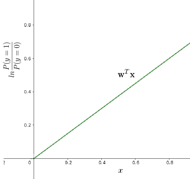
The logistic function above is a nonlinear transformation of the linear function \(\mathbf{w}^T \mathbf{x}\), and is usually hard to interpret. Therefore, we want to convert the above nonlinear relationship between \(\mathbf{x}\) and \(\mathbf{y}\) to a linear relationship. A good way to obtain such linear interpretation is to use the Odds ratio.
Odds ratio is a very popular measure in mathematics, and it refers to the ratio of the probability that an event (say \(\alpha\)) will occur, to probability that \(\alpha\) will not occur. In our case of binary classification, we can define odds ratio as:
\begin{equation}
Odds = \frac{P(y=1)}{P(y=0)}\tag{7}
\end{equation}
Please note that if the odds ratio is \(> 1\), then the output is more likely to be \(1\), and if odds ratio \(< 1\), the output is more likely to be \(0\). If odds ratio \(=1\), then the output is equally likely to be \(0\) or \(1\).
Using the value of \(P(y=1)\) from Equation (6), we can compute odds ratio as follows:
\begin{equation}
Odds = \frac{P(y=1)}{1-P(y=1)} = \frac{1}{1+e^{-\mathbf{w}^T \mathbf{x}}} \div (1-\frac{1}{1+e^{-\mathbf{w}^T \mathbf{x}}})
\end{equation}
\begin{equation}
Odds = \frac{1}{1+e^{-\mathbf{w}^T \mathbf{x}}} \div \frac{1+e^{-\mathbf{w}^T \mathbf{x}}-1}{1+e^{-\mathbf{w}^T \mathbf{x}}}
\end{equation}
\begin{equation}
Odds = \frac{1}{1+e^{-\mathbf{w}^T \mathbf{x}}} \div \frac{e^{-\mathbf{w}^T \mathbf{x}}}{1+e^{-\mathbf{w}^T \mathbf{x}}} = \frac{1}{1+e^{-\mathbf{w}^T \mathbf{x}}} \times \frac{1+e^{-\mathbf{w}^T \mathbf{x}}}{e^{-\mathbf{w}^T \mathbf{x}}}
\end{equation}
\begin{equation}
Odds = \frac{1}{e^{-\mathbf{w}^T \mathbf{x}}} = e^{\mathbf{w}^T \mathbf{x}}\tag{8}
\end{equation}
taking the log of both sides, we get:
\begin{equation}
ln(Odds) = \mathbf{w}^T \mathbf{x}= logit(\mathbf{y})\tag{9}
\end{equation}
The logarithm of odds is called logit, and it expresses the linear relationship between predictor \(x\), and discrete target variable \(y\).
3. Cost Function
[watch video]
Let us review the cost function (also known as error function) of linear regression:
\begin{equation}
E(\mathbf{w}) = \frac{1}{N} \sum\limits_{i=1}^N [y^{(i)}-f(x^{(i)},\mathbf{w})]^2\tag{10}
\end{equation}
where the error here is defined as the sum of differences between training examples \(y^{(i)}\) and the regression line defined by function \(f(x^{(i)},\mathbf{w})\).
In logistic regression, we can use the same definition of cost function, with replacing the linear hypothesis \(f(x^{(i)},\mathbf{w})\) with the new logistic hypothesis \(g(x^{(i)},\mathbf{w})\) in Equation (6):
\begin{equation}
E(\mathbf{w}) = \frac{1}{N} \sum\limits_{i=1}^N [y^{(i)}-g(x^{(i)},\mathbf{w})]^2; \quad\quad where\quad g(x^{(i)},\mathbf{w}) = \frac{1}{1+e^{-\mathbf{w}^T \mathbf{x}^{(i)}}}\tag{11}
\end{equation}
As we know, we want to minimize the error function, meaning we want to compute the derivatives of error function, and solve equations: \(\nabla E(\mathbf{w})= 0\) for each coefficient in \(\mathbf{w}\).
the following plot shows an example of logistic function and it’s first derivative.
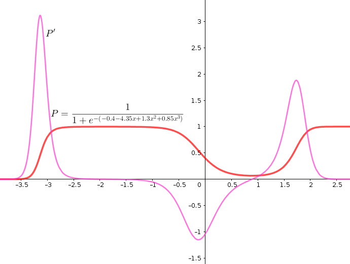
As we can understand from the plot, the derivative of logistic function \(P’\) is non-convex (i.e. has many trends), which means accordingly it has many local minimums. This is problematic when applying algorithm like gradient descent, as the algorithm may converge to a local minimum and generate inaccurate classifier.
Therefore, we need a convex cost function, such that we guarantee the global minimum conversion when computing the gradient. To solve to this problem, we use the concept of likelihood.
3.1 Likelihood Function
Let us transform our understanding of fitting a function, from minimizing the error (in regression problems) to maximizing the cost (in classification problems).
In order to maximize the cost (or penalty) of a probabilistic model that mis-classifies a training example \(y^{(i)}\) (e.g. classify \(y^{(i)}\) as \(0\) (Female) while its true value is \(1\) (Male), or vice versa, let us first define our correct probabilistic model.
\begin{equation}
P(y|\mathbf{x};\mathbf{w}) = \begin{cases}
g(\mathbf{x},\mathbf{w}), & \mbox{if } y=1 \\
1-g(\mathbf{x},\mathbf{w}), & \mbox{if } y=0
\end{cases}
\quad \quad ;g(\mathbf{x},\mathbf{w}) = P(y=1)\tag{12}
\end{equation}
Equation (12) is actually the probability mass function (pmf) of the well-known Bernoulli distribution, and we can write it in one line as:
\begin{equation}
P(y|\mathbf{x};\mathbf{w}) = (g(\mathbf{x},\mathbf{w}))^y \times (1-g(\mathbf{x},\mathbf{w}))^{1-y}\tag{13}
\end{equation}
In Equation (13), the vector of predictors \(\mathbf{x}\) is known, and the target variable \(y= \{0,1\}\) is also known, but vector of coefficients \(\mathbf{w}\) is unknown.
If we assumed that the target samples \(y\) are independently distributed (like the case of genders), then the function of coefficients \(\mathbf{w}\) given values of \(\mathbf{x}\) is called the Likelihood function, and is defined as :
\begin{equation}
L(\mathbf{w}|\mathbf{x}) = P(\mathbf{y}|\mathbf{x};\mathbf{w}) = P(\mathbf{x}|\mathbf{w})\tag{14}
\end{equation}
Please note that, although Equations (13) and (14) are equivalent, they have quite different interpretations. The right-hand term in Equation (14) represent the distribution (or probability) of random variable \(\mathbf{x}\), parametrized by coefficients \(\mathbf{w}\), while the likelihood function on the left-hand side is a function of coefficients \(\mathbf{w}\) given predictors \(\mathbf{x}\).
Following the theory of probabilities, and because our target samples \(y\) are independently distributed, the probability of simultaneous occurrence of \(y\) values is the product of the probabilities of occurrence of each of these values individually:
\begin{equation}
L(\mathbf{w}|\mathbf{x}) = \prod_{i=1}^N P(\mathbf{y^{(i)}}|\mathbf{x^{(i)}};\mathbf{w}) = \prod_{i=1}^N (g(x^{(i)},\mathbf{w}))^{y^{(i)}} \times (1-g(x^{(i)},\mathbf{w}))^{1-{y}^{(i)}}\tag{15}
\end{equation}
The product of many probabilities is not preferable from computational point of view. As you may guess, if we multiply two numbers between \(0\) and \(1\), the output is rather smaller than either of them. This may cause the likelihood \(L(\mathbf{w}|\mathbf{x})\) to approach zero and vanish quickly. Instead, we want to replace the product with summation. Therefore, we take the logarithm of Equation (15):
\begin{equation}
\ell(\mathbf{w})= log(L(\mathbf{w}|\mathbf{x})) = \sum_{i=1}^N {y^{(i)}}\: log(g(x^{(i)},\mathbf{w})) + (1-{y}^{(i)})\: log(1-g(x^{(i)},\mathbf{w}))\tag{16}
\end{equation}
In addition to the computational advantage of Equation (16), the log likelihood function is a convex function, meaning that optimizing it’s first derivative is guaranteed to approach the global minimum (or maximum).
Now the question would be, should we minimize \(\ell(\mathbf{w})\) or maximize it? To answer this question, let us divide Equation (16) into 2 parts, depending on the value of \(y^{(i)}\):
\begin{equation}
\ell(\mathbf{w}) = \begin{cases}
log(g(x^{(i)},\mathbf{w})), & \mbox{if } y^{(i)}=1 \\
log(1-g(x^{(i)},\mathbf{w})), & \mbox{if } y^{(i)}=0
\end{cases}\tag{17}
\end{equation}
Let us plot both cases and see what is happening:
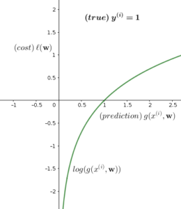
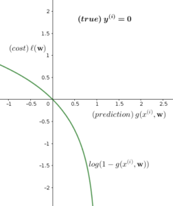
As the left plot shows, if the training example \(y^{(i)}=1\) and prediction \(g(x^{(i)},\mathbf{w})= 1\) (correct prediction), then the cost function \(\ell(\mathbf{w}) = 0\). As prediction moves to \(0\) (wrong prediction), the cost function \(\ell(\mathbf{w})\) approaches to \(-\infty\). The same case when \(y^{(i)}=0\) (right plot), if the prediction \(g(x^{(i)},\mathbf{w})= 0\), the cost function \(\ell(\mathbf{w}) = 0\), and as the prediction moves to \(1\), the cost function moves to \(-\infty\).
Now, as we have a logic cost function for logistic regression, the next step is to maximize the likelihood function \(\ell(\mathbf{w})\) and solve it for each coefficient \(w \in \mathbf{w}\) (because the error increases as we move to \(-\infty\)). This process is known as maximum likelihood estimation (MLE). Note here that maximizing the likelihood function is equivalent to minimizing the error function in regression methods.
If you want to minimize \(\ell(\mathbf{w})\) rather than maximizing it, all you need to do is changing the sign of Equation (17) to \((-)\), and you get the correct answer. Below are the plots of \(-\ell(\mathbf{w})\):
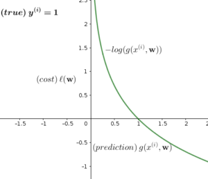
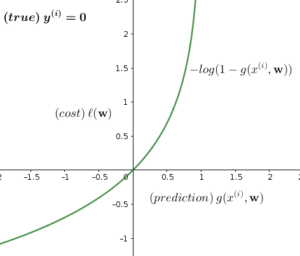
In the above plots, the cost function \(\ell(\mathbf{w})\) is approaching \(\infty\) if the prediction function \(g(x^{(i)},\mathbf{w})\) mis-classifies the target variable \(y^{(i)}\), and accordingly we need to minimize \(\ell(\mathbf{w})\) to obtain correct classifications.
3.2 Compute Derivatives of Likelihood Function (\(∇\ell(w)\))
Let us compute the derivatives of likelihood function with respect to each coefficient \(w_j\):
\begin{equation}
\frac{\partial\ell(\mathbf{w})}{\partial w_j}= \sum_{i=1}^N \frac{\partial[{y^{(i)}}\: log(g(x^{(i)},\mathbf{w})) + (1-{y}^{(i)})\: log(1-g(x^{(i)},\mathbf{w}))]}{\partial w_j}\tag{18}
\end{equation}
Following the rules of differentiating a logarithmic function, we know that:
\begin{equation}
f(x) = log(x) \quad\quad \Rightarrow \quad\quad f'(x) = \frac{1}{x} \frac{\partial f(x)}{\partial x}
\end{equation}
Applying this rule to Equation (18), we get:
\begin{equation}
\begin{split}
\frac{\partial\ell(\mathbf{w})}{\partial w_j}&= \sum_{i=1}^N \Big[ \frac{y^{(i)}}{g(x^{(i)},\mathbf{w})}\times\frac{\partial\,g(x^{(i)},\mathbf{w})}{\partial w_j}\Big] + \Big[ \frac{1-y^{(i)}}{1-g(x^{(i)},\mathbf{w})} \times\frac{\partial\,(-g(x^{(i)},\mathbf{w}))}{\partial w_j}\Big]\\
&= \sum_{i=1}^N \frac{y^{(i)}}{g(x^{(i)},\mathbf{w})}\times\frac{\partial\,g(x^{(i)},\mathbf{w})}{\partial w_j} – \frac{1-y^{(i)}}{1-g(x^{(i)},\mathbf{w})} \times\frac{\partial\,g(x^{(i)},\mathbf{w})}{\partial w_j}
\end{split}\tag{19}
\end{equation}
Let us expand the derivative component in Equation (19) using Chain Rule:
\begin{equation}
\frac{\partial\,g(x^{(i)},\mathbf{w})}{\partial w_j}= \frac{\partial\,g(f(x^{(i)},\mathbf{w}))}{\partial w_j} = \frac{\nabla\,g(x^{(i)},\mathbf{w})}{\nabla\,f(x^{(i)},\mathbf{w})}\times\frac{\partial\,f(x^{(i)},\mathbf{w})}{\partial w_j}\tag{20}
\end{equation}
Remember that:
\begin{equation}
g(x^{(i)},\mathbf{w}) = \frac{1}{1+e^{-\mathbf{w}^T x^{(i)}}}
\end{equation}
\begin{equation}
f(x^{(i)},\mathbf{w})= \mathbf{w}^T x^{(i)}
\end{equation}
Let us substitute the linear component \(\mathbf{w}^T x^{(i)}\) of our logistic hypothesis with letter \(z\) for simplicity. Accordingly, our hypothesis component \(g(x^{(i)},\mathbf{w})\) in equation (20) will become \(g(z)\). Then we write our hypothesis again with the simplified notation:
\begin{equation}
g(x^{(i)},\mathbf{w}) = \frac{1}{1+e^{-\mathbf{w}^T x^{(i)}}} = \frac{1}{1+e^{-z}} = g(z)\tag{21}
\end{equation}
By applying both reciprocal and exponential rules of differentiation:
\begin{equation}
f(x) = \frac{-1}{x} \quad\quad \Rightarrow \quad\quad f'(x) = \frac{1}{x^2} \quad\quad\textrm{reciprocal rule}
\end{equation}
\begin{equation}
f(x) = e^x \quad\quad \Rightarrow \quad\quad f'(x) = e^x \quad\quad\textrm{exponential rule}
\end{equation}
we compute the two derivative terms on the right-hand side of Equation (20) as follows:
\begin{equation}
\frac{\nabla\,g(x^{(i)},\mathbf{w})}{\nabla\,f(x^{(i)},\mathbf{w})} = \frac{\nabla g(z)}{\nabla z} = \frac{1}{(1+e^{-z})^2} (e^{-z})
= \frac{1}{1+e^{-z}}\times \frac{e^{-z}}{1+e^{-z}} = \frac{1}{1+e^{-z}}\times \frac{1+e^{-z}-1}{1+e^{-z}}
\end{equation}
\begin{equation}
\frac{\nabla g(z)}{\nabla z} = \frac{1}{(1+e^{-z})}\times (1 – \frac{1}{1+e^{-z}})
\end{equation}
\begin{equation}
\frac{\nabla g(z)}{\nabla z} = g(z)(1-g(z))\tag{22}
\end{equation}
And the second term:
\begin{equation}
\frac{\partial\,f(x^{(i)},\mathbf{w})}{\partial w_j} = \frac{\partial(\mathbf{w}^T x^{(i)})}{\partial w_j} = \frac{\partial(w_j x^{(i)})}{\partial w_j}= x^{(i)}\tag{23}
\end{equation}
By substituting the right-hand side derivative terms in Equation (20) with their values in Equations (22) and (23), we get:
\begin{equation}
\frac{\partial\,g(x^{(i)},\mathbf{w})}{\partial w_j}= \frac{\partial\,z}{\partial w_j} = g(z)(1-g(z)) x^{(i)}\tag{24}
\end{equation}
Now we use the partial derivative in Equation (24) to solve Equation (19):
\begin{equation}
\frac{\partial\ell(\mathbf{w})}{\partial w_j} = \sum_{i=1}^N \frac{y^{(i)}}{g(z)}g(z)(1-g(z))x^{(i)} – \frac{1-y^{(i)}}{1-g(z)} g(z)(1-g(z))x^{(i)}\tag{25}
\end{equation}
\begin{equation}
\frac{\partial\ell(\mathbf{w})}{\partial w_j} = \sum_{i=1}^N [y^{(i)}(1-g(z)) – (1-y^{(i)})g(z)]x^{(i)}
\end{equation}
\begin{equation}
\frac{\partial\ell(\mathbf{w})}{\partial w_j} = \sum_{i=1}^N (y^{(i)} – y^{(i)} g(z))- g(z)+y^{(i)} g(z))x^{(i)}
\end{equation}
\begin{equation}
\frac{\partial\ell(\mathbf{w})}{\partial w_j} = \sum_{i=1}^N (y^{(i)}- g(z))x^{(i)} = \sum_{i=1}^N [y^{(i)}- g(x^{(i)},\mathbf{w})]x^{(i)}\tag{26}
\end{equation}
Now, let us refresh our memories with the derivative of error function for linear regression, it looks like this:
\begin{equation}
\frac{\partial E(\mathbf{w})}{\partial w_j}= \sum\limits_{i=1}^N [y^{(i)} – f(x^{(i)},\mathbf{w})] x^{(i)}\tag{27}
\end{equation}
As you may notice, the error function of linear regression (Equation (27)) has the same definition as the likelihood function of logistic regression (Equation (26)). The only difference is between the linear hypothesis of linear regression \(f(x^{(i)},\mathbf{w})\) and the logistic hypothesis of logistic regression \(g(x^{(i)},\mathbf{w})\).
4. No Closed-Form Solution
[watch video]
Our cost function is build upon the following logistic hypothesis (Equation (3)):
\begin{equation}
g(\mathbf{x},\mathbf{w}) = \frac{1}{1+e^{-\mathbf{w}^T \mathbf{x}}}\tag{28}
\end{equation}
The above hypothesis is transcendental equation, as it contains exponential component \(e^{-\mathbf{w}^T \mathbf{x}}\). This type of equations has no closed-form solution.
5. Gradient Descent Algorithm
In order to find the list of coefficients of our logistic hypothesis, the above cost function (i.e. log likelihood function) is plugged in the gradient descent algorithm instead of the hypothesis function of linear regression. The algorithm will looks like this.
Algorithm1 GradientDescent(\(\ell(\mathbf{w}),\mathbf{w},\eta\))
- Input:
- \(\ell(\mathbf{w})\): cost function
- \(\mathbf{w}\): initial values of coefficients vector
- \(\eta\): learning rate
- Output:
- \(\mathbf{w}\): updated values of coefficients vector
- Procedure:
- repeat
- \(w_j=w_j – \eta \frac{\partial (-\ell(\mathbf{w}))}{\partial w_p}, \forall w_j \in \mathbf{w}\)
- until \(\nabla \ell(\mathbf{w})= 0\)
- return \(\mathbf{w}\)
In the above algorithm, the cost function is minimized. If you want to maximize it, you should change it’s sign to \((+)\) in step 8.A., and the algorithm’s name will be changed to gradient ascent (see below):
Algorithm2 GradientAscent(\(\ell(\mathbf{w}),\mathbf{w},\eta\))
- Input:
- \(\ell(\mathbf{w})\): cost function
- \(\mathbf{w}\): initial values of coefficients vector
- \(\eta\): learning rate
- Output:
- \(\mathbf{w}\): updated values of coefficients vector
- Procedure:
- repeat
- \(w_j=w_j + \eta \frac{\partial (\ell(\mathbf{w}))}{\partial w_p}, \forall w_j \in \mathbf{w}\)
- until \(\nabla \ell(\mathbf{w})= 0\)
- return \(\mathbf{w}\)
6. Make Predictions
After running the gradient descent (or ascent) algorithm, and obtain estimations of coefficients \(\mathbf{w}\), you need to use these coefficients to estimate the probability of \(y\). But, how you will do this?
In order to obtain probabilities of \(y\), you need to solve the logit Equation (9) for \(p\):
\begin{equation}
log\frac{P(y=1)}{P(y=0)} = e^{-\mathbf{w}^T \mathbf{x}}\tag{29}
\end{equation}
Or simply:
\begin{equation}
log\frac{p}{1-p} = e^{-\mathbf{w}^T \mathbf{x}}\tag{30}
\end{equation}
Solving Equation (30) for \(p\) gives you:
\begin{equation}
p = \frac{e^{-\mathbf{w}^T \mathbf{x}}}{1 + e^{-\mathbf{w}^T \mathbf{x}}}\tag{31}
\end{equation}
The output of Equation (31) is you predictions of \(y\).
7. Newton’s Method
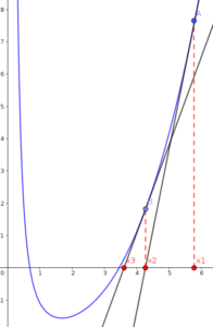
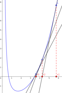
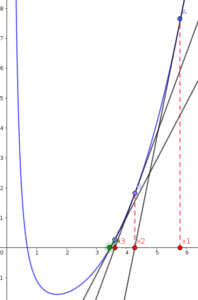
Newton’s method is a very simple and effective way of finding roots of a function (i.e. points at which function equal to \(0\)). It is widely used in machine learning to minimize error functions. Let us take an example of the following function:
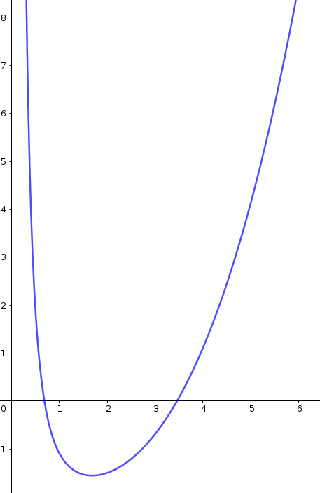
Newton’s method starts by selecting a random value of function (say \(x_1\)), and computes the tangent of the function at this value:
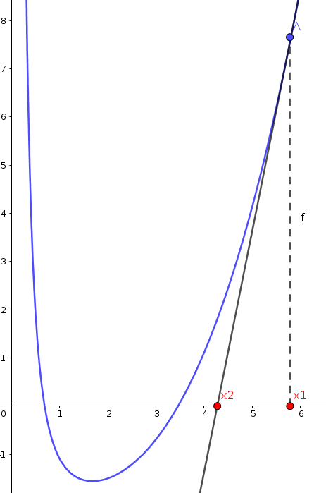
The tangent of \(f(x_1)\) intersects with \(X\) axis at new value (say \(x_2\)). If we assume the distance between \(x_1\) and \(x_2\) is \(\Delta x\), then we can say that:
\begin{equation}
x_2 = x_1 – \Delta x\tag{32}
\end{equation}
Now we want to measure \(\Delta x\). From the following figure, it turns out that \(\Delta x\) equals to \(\frac{f(x_1)}{f'(x_1)}\):
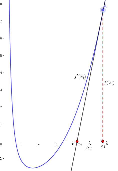
By substituting \(\Delta x\) in Equation (32) with its value, we can compute \(x_2\) as:
\begin{equation}
x_2 = x_1 – \frac{f(x_1)}{f'(x_1)}\tag{33}
\end{equation}
if we repeat this process several times, we will reach to a value of \(x\) close to the root (\(x\) at \(y=0\)) (see following plots):
As mentioned earlier above, the function we want to minimize (or maximize) in logistic regression, is the derivative of log likelihood function \(\ell(\mathbf{w})\). Therefore, we can apply Newton’s method by using the following update of each coefficient \(w_j\) in vector \(\mathbf{w}\):
\begin{equation}
w_j = w_j – \frac{\ell'(\mathbf{w})}{\ell”(\mathbf{w})};\quad \quad \quad \quad \forall w_j \in \mathbf{w}\tag{34}
\end{equation}
In Section 3.2 we computed the first derivative of log likelihood function \(\ell'(\mathbf{w})\). Now, let us compute the second derivative \(\ell”(\mathbf{w})\).
7.1 Compute Second Derivative of Log Likelihood Function (\(\ell”(\mathbf{w})\))
Let us recall the value of first derivative in Equation (26)
\begin{equation}
\ell'(\mathbf{w}) = \frac{\partial\ell(\mathbf{w})}{\partial w_j} = \sum_{i=1}^N [y^{(i)}- g(x^{(i)},\mathbf{w})]x^{(i)}
\end{equation}
In order to obtain the second derivative, we compute the derivative of \(\ell'(\mathbf{w})\) with respect to \(w_j\):
\begin{equation}
\ell”(\mathbf{w}) = \frac{\ell'(\mathbf{w})}{\partial w_j} = \frac{\partial(\sum_{i=1}^N [y^{(i)}- g(x^{(i)},\mathbf{w})]x^{(i)})}{\partial w_j}\tag{35}
\end{equation}
\begin{equation}
\ell”(\mathbf{w}) = \frac{\partial(\sum_{i=1}^N [x^{(i)} y^{(i)}- x^{(i)} g(x^{(i)},\mathbf{w})])}{\partial w_j} = \frac{-\sum_{i=1}^N \partial(x^{(i)} g(x^{(i)},\mathbf{w}))}{\partial w_j}\tag{36}
\end{equation}
\begin{equation}
\ell”(\mathbf{w}) = -\sum_{i=1}^N x^{(i)} \frac{\partial(g(x^{(i)},\mathbf{w}))}{\partial w_j}\tag{37}
\end{equation}
By substituting the component \(\frac{\partial(g(x^{(i)},\mathbf{w}))}{\partial w_j}\) with its value defined in Equation (24), we get:
\begin{equation}
\ell”(\mathbf{w}) = -\sum_{i=1}^N x^{(i)} g(x^{(i)},\mathbf{w})(1-g(x^{(i)},\mathbf{w})) {x^{(i)}}^T\tag{38}
\end{equation}
The formula of Equation (38) is called the Hessian Matrix, and it can be written into a matrix form as follows:
\begin{equation}
\mathbf{H}^{(i)} = \mathbf{X}\mathbf{G}\mathbf{X}^T\tag{39}
\end{equation}
If we consider that we have \(M\) predictor variables, then we compute Hessian components as follows:
\begin{equation}
\mathbf{G}
= \begin{bmatrix}
g(x_0^{(i)},w_0)(1-g(x_0^{(i)},w_0)) & 0 & 0 \\
0 & g(x_1^{(i)},w_1)(1-g(x_1^{(i)},w_1)) & 0 \\
… & … & … \\
0 & 0 & g(x_M^{(i)},w_M)(1-g(x_M^{(i)},w_M))
\end{bmatrix}_{1+M\times1+M}
\end{equation}
\begin{equation}
\mathbf{X} = \begin{bmatrix}
1 \\
x_1^{(i)} \\
x_2^{(i)} \\
\vdots \\
x_M^{(i)} \\
\end{bmatrix}_{1+M\times1}
\end{equation}
\begin{equation}
\mathbf{X}^T =
\begin{bmatrix}
1 & x_1^{(i)} & x_2^{(i)} & …&x_M^{(i)}
\end{bmatrix}_{1\times1+M}
\end{equation}
By multiplying the above three matrices, we get a Hessian matrix with \([1+M\times1+M]\) dimensions. After computing \(\mathbf{H}^{(i)}\), we can apply Newton’s method in the coefficients’ updates as:
\begin{equation}
w_j = w_j – \mathbf{H}^{-1}\: \ell'(\mathbf{w})\tag{40}
\end{equation}
8. Multivariate Logistic Regression
If we want to use multiple independent variables \(\mathbf{x} = \{x_1, x_2, …,x_k\}\), we adopt the vector form of linear hypothesis of logistic function to our calculations (see Equations (5) and (6) above).
9. Implementation in Python
You can find python implementations of the above algorithms on my GitHub.


When I initially commented I clicked the “Notify me when new comments are added” checkbox and now each time a comment is added I get four e-mails with the same comment. Is there any way you can remove me from that service? Thank you!
Hallo! Sorry for this inconsistency, please try again and I hope the error is fixed
I loved this post! Nice article I visit your blog fairly often and you’re
always coming out with some quality stuff. I posted
this on my Facebook Page and my friends loved it! Keep it up!.
🙂
Thanks a lot for the blog.
You’re welcome!