Predictive Data Analytics With Apache Spark (Part 6 Binary Classification)
January 20, 2019

1. Select Features
The main task in this article is to build binary classifiers that can differentiate between two time frames during Engine’s life; the Alarm Zone (1-15 runs before Engine’s failure) and the Normal Zone (longer than 15 runs before Engine’s failure).
The first step toward building classifiers is to visualize data features and select the most expressive ones to be learned by the classifiers.
The first set of features we want to visualize is the set of standardized features of both train and test datasets. The following figure displays the standardized features of Engine #15 for train dataset (left) and test dataset (right).
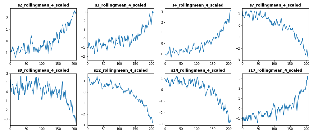
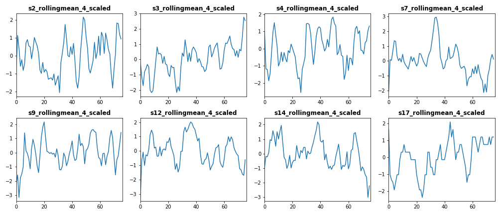
From the above figure we conclude that features [s3_rollingmean_4_scaled, s4_rollingmean_4_scaled, s7_rollingmean_4_scaled, s12_rollingmean_4_scaled, and s17_rollingmean_4_scaled] have common trend in both train and test dataset. Therefore, we include these features as independent features in our classifiers.
The second set of features we want to visualize is the set of standardized PC features of both train dataset (left) and test dataset (right), which are plotted below.
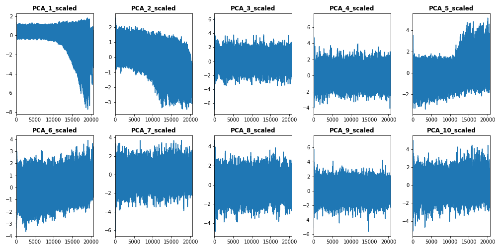
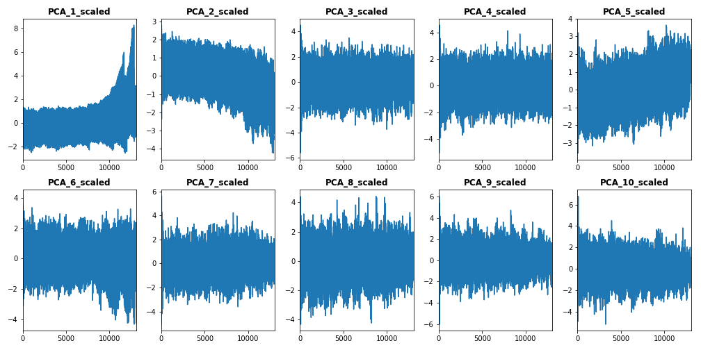
From this subset of features, we select the first standardized PCs [PCA_1_scaled to PCA_5_scaled] to be included them in our train vector.
2. Build Features Vector of Train Dataset
After selecting features for classification, we build our train data vector using the following code:
# select features to be used into classification algorithms
train = train_df.select(train_df["s3_rollingmean_4_scaled"],train_df["s4_rollingmean_4_scaled"],
                        train_df["s7_rollingmean_4_scaled"],train_df["s12_rollingmean_4_scaled"],
                        train_df["s17_rollingmean_4_scaled"],train_df["PCA_1_scaled"],
                        train_df["PCA_2_scaled"],train_df["PCA_3_scaled"],train_df["PCA_4_scaled"],
                        train_df["PCA_5_scaled"],train_df["label1"])

# build train features vector
train_vector = train.rdd.map(lambda x: [x[10], Vectors.dense(x[0:10])]).toDF(['label','features'])
3. Logistic Regression
3.1 Initialize Logistic Regression Instance
The first binary classifier in this tutorial is the Logistic Regression classifier. We start building the classifier by initializing an instance of LogisticRegression() function:
from pyspark.ml.classification import LogisticRegression
# init log regression object
lr = LogisticRegression(featuresCol='features', labelCol='label', family='binomial',  maxIter=10)
As we explained in the previous Post of this tutorial, we add the names of independent and target variables to the classifier function.
3.2 Cross Validation
Cross validation is a common procedure taken within classification algorithms to avoid model overfitting against certain test data subsets. In order to apply cross validation in Apache Spark, we firstly need to build a parameter grid object. Parameter grids enables a given classifier to try out different input parameters’ settings and optimize the accuracy between each combination of them. The following code snippet builds a parameter grid that loop over a list of values of regression and elastic search parameters of logistic regression.
from pyspark.ml.tuning import ParamGridBuilder
# init parameter grid for log rgression params
paramGrid = ParamGridBuilder()
             .addGrid(lr.regParam, [0.1, 0.3]) # regularization parameter
             .addGrid(lr.elasticNetParam, [0.0]) # Elastic Net Parameter
             .build()
Secondly, we set the classifier evaluator, using BinaryClassificationEvaluator() function.
from pyspark.ml.evaluation import BinaryClassificationEvaluator
# create evaluator
evaluator = BinaryClassificationEvaluator(rawPredictionCol="label")
Thirdly, we create CrossValidator() object and pass model, parameter grid, and evaluation instances to it. In this step, we can set the number of folds we wish to use in our cross validation procedure. In the below code we use 10 folds.
from pyspark.ml.tuning import CrossValidator
# create cross validation object
crossval = CrossValidator(estimator=lr,
                          estimatorParamMaps=paramGrid,
                          evaluator=evaluator,
                          numFolds=10)
3.3 Fit Log. Regression Model to Training Data Vector
After initializing the cross validation object, we use it to fit our log. regression model to the train vector.
# run cross-validation, and choose the best set of parameters.
cvModel = crossval.fit(train_vector)
3.4 Get Predictions
After fitting the model, we evaluate it using confusion matrix. This means we need to extract true & predicted labels out of the model. The following function achieves this goal.
def get_prediction_lists(prediction_df):
    '''
    this function returns true & predicted labels as Python lists, plus array of predictions,
    using Spark prediction DF as input

    INPUTS:
    @prediction_df: Spark DF of classifier predictions

    OUTPUTS:
    @l1: list of true labels
    @l2: list of predicted labels
    @m1: array of predictions
    '''

    l1 = map(int, get_col_as_list(prediction_df, "label"))
    l2 = map(int, get_col_as_list(prediction_df, "prediction"))
    m1 = get_col_as_nparray(prediction_df, "probability")

    return l1, l2, m1
3.5 Build Confusion Matrix
Once we obtain true and predicted data labels using the above function, we can build our confusion matrix using confusion_matrix() function.
from sklearn.metrics import confusion_matrix
# get confusion matrix
logreg_matrix = confusion_matrix(labels, preds)
Confusion matrix is a very effective tool for measuring the accuracy of binary and multi classifiers. It is used to calculate very common evaluation metrics such as precision, recall, and F1.
4. Decision Tree
The second binary classifier in this Post is the Decision Tree classifier. To build the classifier we follow the same steps as of Log. Regression classifier in the previous Section.
from pyspark.ml.classification import DecisionTreeClassifier
# init decision tree object
dt = DecisionTreeClassifier(featuresCol='features', labelCol='label')

# add empty parameter grid
paramGrid = ParamGridBuilder()\
            .addGrid(dt.maxDepth, [4,5])\
            .build()

# create evaluator
evaluator = BinaryClassificationEvaluator(rawPredictionCol="label", metricName="areaUnderROC")

# create cross validation object
crossval = CrossValidator(estimator=dt,
                          estimatorParamMaps=paramGrid,
                          evaluator=evaluator,
                          numFolds=5)

# run cross-validation, and choose the best set of parameters.
cvModel_dt = crossval.fit(train_vector)

# make predictions on test data
prediction_dt = cvModel_dt.transform(test_vector)

# get labels, predictions, and probabilities as python lists and nparrays
labels, preds, probs = get_prediction_lists(prediction_dt)

# get confusion matrix
dt_matrix = confusion_matrix(labels, preds)
5. Random Forest
The third classifier in this article is the Random Forest classifier. To build the classifier we follow the same steps as of the above classifiers.
from pyspark.ml.classification import RandomForestClassifier
# init random forest object
rf = RandomForestClassifier(featuresCol='features', labelCol='label')

# add parameter grid
paramGrid = ParamGridBuilder().addGrid(rf.numTrees,[10,20]).build()

# create evaluator
evaluator = BinaryClassificationEvaluator(rawPredictionCol="label", metricName="areaUnderROC")

# create cross validation object
crossval = CrossValidator(estimator=rf,
                          estimatorParamMaps=paramGrid,
                          evaluator=evaluator,
                          numFolds=5)

# run cross-validation, and choose the best set of parameters.
cvModel_rf = crossval.fit(train_vector)

# make predictions on test data
prediction_rf = cvModel_rf.transform(test_vector)

# get labels, predictions, and probabilities as python lists and nparrays
labels, preds, probs = get_prediction_lists(prediction_rf)

# get confusion matrix
rf_matrix = confusion_matrix(labels, preds)
6. Compare Classifiers
After building and evaluating the above three classifiers, we want to compare them using different evaluation metrics. The following figure shows the performance of each classifier over 10 random selected engines, using Accuracy, Macro Precision, Macro Recall, and Macro F1 metrics.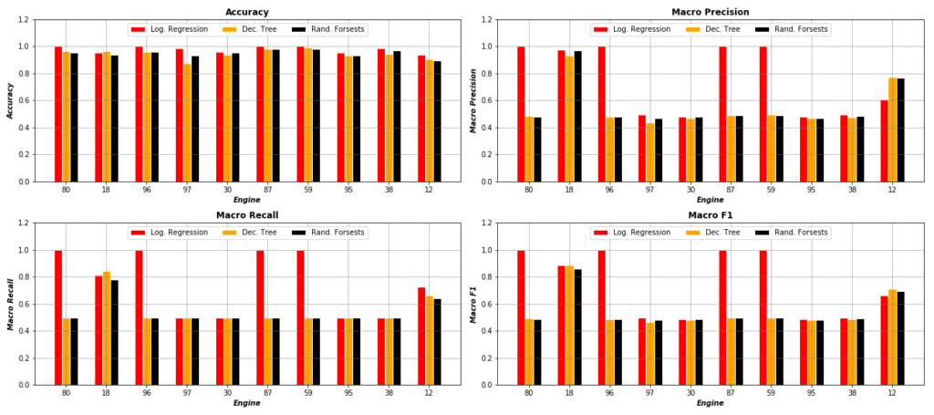 As the figure displays, it is clear that Log. Regression classifier outperforms both Decision Tree and Random Forest in most of test engines.
7. Full Code
The code of this tutorial can be found in my Github under this link.