


As another example, suppose you have a list of heights (in inches) of random sample of students in a high school: \(heights=\{65.78, 71.52, 69.40, 68.22\}\), and you want to model these observations using a continuous function. The first logical way of thinking is to assume the heights vector is following a normal probability distribution, and compute both mean and variance of the sample data to visualize your probability function: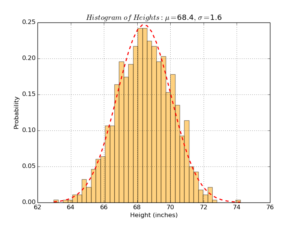
Expressing uncertainty plays basic role in machine learning, as it enables us to make predictions of events which haven’t happened yet (e.g. earthquakes).
2.3 Exploring Statistics
The third benefit of probability distributions is that once you define the distribution your data is drawn from, you can easily find interesting statistics (or facts) about your data. For example, given the above heights example, once you found a probability distribution (e.g. normal distribution) to express it, you can answer questions like: what is the maximum height? minimum height? variance between heights? most common height? and so on.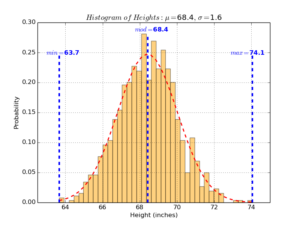
2.4 Data Imputation
Another common application of probability distributions is to impute (i.e. fill-in) missing values in your data. Suppose for example you got a vector of heights, but with some missing values:
\begin{equation} heights=\{65.78, 71.52, ?, 68.22, ?, 68.70, ?, 70.01\}\end{equation} A common technique to fill-in these missing values is to draw these missing points multiple times using one probability distribution with different parameter settings, analyze multiple versions of your data, and finally integrate all versions into one final version (maybe with minimum variance or narrowest confidence interval). This technique is called multiple imputation, and it is widely used to fill-in missing data values.
2.5 Making Predictions
The fifth usage of probability distributions is to make predictions of events and hypotheses, using our believes and/or some historical data. Common approaches of calculating predictions (or guesses) using probability distributions are Bayesian and Frequentist Inferences.
3. Components
There are multiple components of probability distributions, that outline their functionalities and applications. Anyone wants to use a distribution should learn about it’s specific components. In the following points, I will try to briefly cover some of the basic components of probability distributions.
3.1 Random Variables
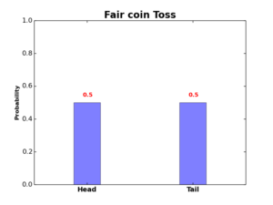
A random variable is a numerical mapping of all possible outcomes of a random process, and a random process is a process we do not know it’s outcome until it occurs. For example, the random variable \(X\) of tossing a fair coin can be expressed as \(X=\{0,1\}\), where the outcome \(Head\) is mapped to 0 and the outcome \(Tail\) is mapped to 1.
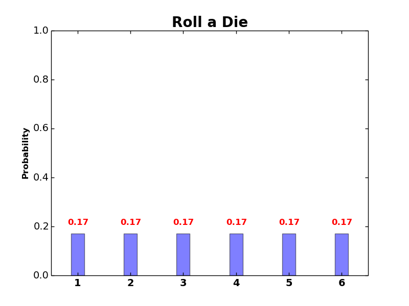
Another example is rolling a die, where random variable \(X\) can be represented by \(X=\{1,2,3,4,5,6\}\), with each side of the die is encoded to its equivalent numerical value in vector \(X\).
As we saw before (in logistic regression post), there are two basic types of data variables: categorical (discrete) and quantitative (continuous). There are also two corresponded types of random variables: continuous and discrete random variables. Each type of random variables is represented by a specific class of probability functions.
3.2 Probability Mass Function (PMF)
Probability Mass Functions (PMF) are functions that describe probability values of discrete random variables \(X\). PMF(\(X\)) must sum up to 1 for all possible values of \(X\).
For example, if we compute the PMF of rolling a die, where random variable \(X=\{1,2,3,4,5,6\}\), we can draw PMF(\(X\)) as follows: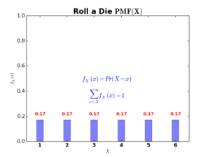
\begin{equation}
f_X(x)=Pr(X= x)\ \ \ and\ \ \ \sum_{x\in X} f_X(x)=1\tag{1}
\end{equation}
A probability mass function (PMF) computes the probability that a random variable \(X\) can take any possible outcome \(x\in X\). In dice example, \(f_X(x=3)=0.17,\ f_X(x=1)=0.17,\ f_X(x=7)=0\). Note that the sum of all possible values of \(x\) equals to 1.
3.3 Probability Density Function (PDF)
As PMF describes probability values of discrete random variables, the probability density function (PDF) describes probability values of continuous random variables. An example of PDF is the one of normal distribution below: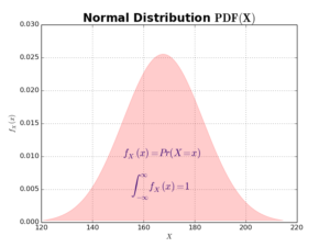 Please note that for PDFs, the area under curve must sum up to 1.
3.4 Cumulative Distribution Function (CDF)
Beside PMF and PDF, there exist a third type of functions for both discrete and continuous variables. These are cumulative distribution functions (CDF). The CDF computes the cumulative probability up to a given value \(x\in X\). In case of discrete random variable, the CDF looks like this: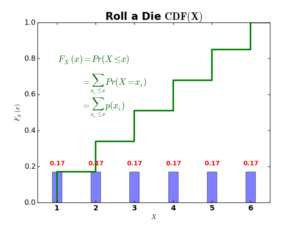
The green stepwise function above represents the CDF of rolling a die, and it is computed as follows:
\begin{equation}
\begin{split}
F_X(x) &=Pr(X\leq x) \\
&=\sum_{x_i\leq x} Pr(X=x_i) \\
&=\sum_{x_i\leq x} p(x_i)
\end{split}\tag{2}
\end{equation}
You can think of \(F_X(x)\) as summing up all probabilities upto value \(x\). For example:
\begin{equation}
F_X(x=3)= \sum_{x_i=1}^3 p(x_i)= 0.17+0.17+0.17=0.51
\end{equation}
For continuous random variables, CDFs using integrals instead of summations, in order to compute the area under continuous PDF curves. The next figure shows an example of the normal distribution CDF.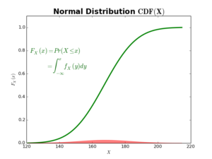
\begin{equation}
\begin{split}
F_X(x) &=Pr(X\leq x) \\
&=\int_{-\infty}^x f_X(y)dy
\end{split}\tag{3}
\end{equation}
where \(y\) is a dummy integration variable.
Please note that for continuous random variables, we integrate PDF(\(x\)) over given limits (say \(\{a,b\}\)) to obtain CDF(\(x\)), and we differentiate CDF(\(x\)) with respect to \(x\) to obtain PDF(\(x\)).